Kalman Filter for Crypto Pairs Trading: Dynamic Hedge Ratios in Python
A beginner-friendly, hands-on guide to dynamic regression, with a reproducible Python experiment.
Imagine you are watching Bitcoin (BTC) and Ethereum (ETH) on a trading dashboard. Both prices have been rising, but today ETH rises noticeably faster. Is ETH suddenly “too expensive” compared with BTC? Is that difference unusual, or is their relationship itself changing?
A chart with two price lines cannot tell you. To make the question measurable, we need a model of how the prices relate, a way to detect changes in that relationship, and a test that does not accidentally use tomorrow’s information to explain yesterday.
This tutorial develops one possible tool: the Kalman filter. We start with intuition and actual numbers, learn enough regression to understand a hedge ratio, and only then build the mathematical model. Finally, we run Python code, examine a labeled synthetic BTC–ETH experiment, and show how to repeat the analysis on actual public market data. We do not claim that the strategy makes money. The code tests relative-price estimation, not live trades or a profitable trading backtest.
You will learn: why correlation is not a trading signal; what a fixed hedge ratio assumes; how a Kalman filter decides whether to trust its previous estimate or new observations; what its equations mean; how to reproduce a causal Python experiment; and which further tests are required before placing a trade.
Who is this for? Python learners, data scientists, and aspiring quantitative analysts. You need basic Python and the idea of an average; we explain logarithms, regression, matrices, and uncertainty as they appear. If you already know ordinary least squares (OLS), you can jump to the Kalman walkthrough. The related Mean Reversion Trading in Python tutorial explores fixed-parameter pairs strategies, z-scores, and transaction-cost-aware backtesting in greater depth.
1. Start with a real question: has ETH moved too far from BTC?
Suppose BTC is trading at $60,000 and ETH at $3,000. One hour later, BTC trades at $61,200 and ETH at $3,090. BTC has risen by 2%; ETH by 3%. You might ask whether ETH has moved more than expected based on BTC.
The naive answer is “ETH rose 1 percentage point more, so short ETH and buy BTC.” That conclusion is premature. Perhaps ETH normally reacts more strongly to broad crypto-market moves. Perhaps the relationship changed after new information. And even if an unusual gap appears, there is no guarantee it closes before trading costs exceed the gain.
We therefore separate three different questions:
- Description: How has ETH usually changed when BTC changes?
- Adaptation: Does that relationship stay constant, or does it drift over time?
- Trading: Even if we can model the relationship, do the deviations reliably reverse after costs and with realistic execution?
This article focuses on questions one and two. The third requires a separate, defensible trading experiment. That distinction is central to quantitative research: a good statistical model is not automatically a good strategy.
A small example of a relative-price expectation
Suppose past data suggest that a 1% BTC change has typically been associated with an approximately 1.4% ETH change. If BTC rises 2%, a simple model would associate that with roughly 2.8% ETH movement. The observed 3% move is only about 0.2 percentage points above that rough expectation—not the full 1 percentage point suggested by comparing raw returns.
This example is deliberately approximate. The regression model below works with log prices, not a regression fitted directly on hourly returns; its beta measures the fitted relationship between levels, and changes in those levels have an approximate percentage interpretation. Whether the remaining gap is statistically unusual depends on its typical variability. And whether it is tradable is a further question still.
2. Three terms you need: correlation, spread, and hedge ratio
Correlation: do the changes tend to move together?
Correlation describes how consistently two sets of movements line up. A high correlation between hourly BTC and ETH returns means they often rise and fall together over those hours. It does not mean their relative price will return to a fixed level. Two assets can be highly correlated while one steadily outperforms the other.
Spread: the difference after accounting for the relationship
If a model expects ETH’s log price to be a function of BTC’s log price, the spread or residual is the observed ETH log price minus the expected value. Think of it as the model’s unexplained difference—not the dollar amount you could directly collect from an exchange.
A spread close to zero means the two prices are near the model’s fitted relationship. A positive spread means ETH’s log price is above what the model predicts at that BTC price. Whether this gap is unusual depends on how much residual noise the model typically sees.
Hedge ratio: how sensitive is the fitted relationship?
The hedge ratio, often written as beta (), describes the fitted sensitivity of ETH’s log price to BTC’s log price. If beta is 1.4, a small 1% change in BTC corresponds to about a 1.4% change in fitted ETH log price, all else equal. That is a descriptive regression coefficient; it is not a promise about tomorrow.
For an illustrative long-spread position, beta can also inform opposite dollar exposures: long ETH and short approximately beta times as much BTC notional, normalized to a chosen gross exposure. But a time-varying beta makes those exposures change, so a real strategy would need rebalancing, turnover and financing costs.
3. Why use log prices instead of raw dollars?
BTC and ETH have very different nominal prices. Taking natural logarithms lets us compare changes in a scale-independent way:
Here
and
are the BTC/USD and ETH/USD prices at observation
.
The symbol
means natural logarithm. You do not have to compute logarithms
by hand: NumPy’s np.log(...) does it.
Why does it help? Because changes in log prices are close to percentage changes for modest moves:
For example, np.log(1.02) is approximately
0.0198, close to 2%. This makes beta interpretable as
an approximate percentage sensitivity when comparing changes. It does
not turn two trending prices into a stationary trading
pair. Logarithms improve the representation; they do not establish
cointegration.
import numpy as np

btc_before, btc_after = 60_000, 61_200
eth_before, eth_after = 3_000, 3_090

print("BTC log return:", np.log(btc_after / btc_before))
print("ETH log return:", np.log(eth_after / eth_before))
4. First build the simpler model: ordinary least squares (OLS)
Before introducing Kalman filtering, imagine fitting one straight-line relationship to historical observations:
Read it in plain English: “The expected ETH log price equals a baseline (alpha) plus beta times the BTC log price, plus an unexplained error.”
- : ETH log price at time .
- : BTC log price at the same time.
- : intercept, a baseline adjustment.
- : slope or hedge ratio.
- : residual, the part not captured by the line.
OLS chooses alpha and beta so the sum of squared residuals over the training observations is as small as possible:
The hat marks an estimate, not the unknown true value. Squaring prevents positive and negative residuals from simply canceling and gives larger errors extra weight.
One tiny numerical example
Suppose an artificial dataset has a BTC regressor equal to and ETH response equal to . The fitted line is exactly : alpha is 3 and beta is 1. Each fitted value matches its observed value, so the residuals are zero. Real market data are noisy, so the residuals will rarely be zero.
We should also center the BTC log prices around their training mean before fitting. This does not change the basic idea, but keeps the intercept and slope numerically easier to estimate:
import numpy as np

# btc_log_train and eth_log_train are 1D NumPy arrays.
origin = btc_log_train.mean()            # TRAINING data only
x_train = btc_log_train - origin
X = np.column_stack([np.ones(len(x_train)), x_train])
alpha, beta = np.linalg.lstsq(X, eth_log_train, rcond=None)[0]
What goes wrong with one fixed beta?
If we fit beta in January and use it unchanged in March, we assume the same relative sensitivity still describes the data. But BTC and ETH may respond differently as conditions evolve. A beta that was reasonable before an important market change can become inaccurate afterward.
Re-running OLS on a short rolling window is one option. It can react to changes, but rolling estimates can jump when an observation enters or leaves the window. The Kalman filter offers a smoother, uncertainty-aware way to adapt, provided we model its assumptions carefully.
5. Kalman filtering without equations: a running estimate with confidence
Imagine trying to estimate the temperature in a room with a slightly noisy thermometer. Yesterday you estimated 20°C, but this morning the thermometer reads 22°C. Should you immediately conclude the true room temperature is 22°C?
Probably not. If the thermometer is noisy, trust the previous estimate more. If the room can heat up quickly, trust the new reading more. The Kalman filter formalizes this balance between what the model already believed and the new evidence.
Our crypto problem uses the same idea, but instead of estimating temperature, we estimate two values that may evolve: alpha and beta. At each observation, the filter:
- Starts with its previous estimates of alpha and beta.
- Predicts the ETH log price using the current observed BTC log price.
- Compares the predicted and observed ETH values; this gap is called the innovation.
- Updates alpha and beta by an amount determined by their uncertainty and the assumed observation noise.
- Stores the updated estimates for the next observation.
The important order is predict first, then observe ETH, then update. If you update with today’s ETH close before claiming to predict that same close, you have leaked information into the reported prediction.
A completely worked one-number example
For intuition, forget alpha and beta for a moment and imagine tracking a single quantity. Your prior estimate is 1.20, and you are somewhat uncertain about it: prior variance 0.05. A new noisy measurement is 1.50, with measurement-error variance 0.20.
The simplified Kalman gain is:
This means the filter applies 20% of the observed surprise to the old estimate:
You do not jump all the way to 1.50; you move from 1.20 to 1.26. If measurements were more reliable, the gain would increase and you would react more strongly. If the earlier estimate were more reliable, the gain would decrease.
This scalar example is a teaching analogy, not the exact two-parameter BTC–ETH filter. Our actual model estimates alpha and beta together, so the gain becomes a two-element vector. But the intuition—adjust estimates in proportion to uncertainty—is identical.
6. Translate that intuition into a state-space model
We now have everything needed for the equations. A state is simply a variable we cannot directly see, but want to estimate. Here the state is a pair of evolving regression coefficients:
Observation equation: what price would our current relationship predict?
There are no hidden tricks in the matrix notation: multiply by and you obtain . The leftover is the observation error. Here is centered BTC log price and is ETH log price.
We model the observation error as having mean zero and variance :
The letter answers: how noisy do we expect the observed ETH value to be around the model’s fitted relationship?
State equation: how can our estimate change through time?
We assume the underlying coefficients move gradually from one observation to the next, with random changes . The matrix expresses how much those coefficients are allowed to drift.
Why two types of noise? describes deviations in observed ETH around its modeled price. describes changes in the relationship itself. If is tiny, alpha and beta barely move. If is too large, they may chase temporary noise and overfit. These quantities must be chosen using training or validation data, not optimized after looking at the final test results.
This is a deliberately simple linear Gaussian random-walk model. Actual crypto markets can have jumps, changing volatility and sudden structural breaks; the model is a starting point, not a complete description of reality.
7. The Kalman equations, one operation at a time
This section contains more symbols, but each corresponds to an action we have already explained. is the estimated uncertainty of our coefficient estimates. The subscript means at time t, using information up to t−1. The subscript means after processing the observation at t.
Step A: predict the next state and its uncertainty
Our starting guess is yesterday’s updated alpha and beta. Because the relationship might drift, we increase our uncertainty by .
Step B: predict ETH given the newly observed BTC price
This is a contemporaneous conditional estimate: at time , BTC’s observed value is supplied to predict ETH’s before updating on ETH’s observed value. It is not a prediction of both BTC and ETH one hour into the future. That difference matters if you later convert the residual into a trading signal.
Step C: calculate the surprise and its uncertainty
The innovation tells us how much the observation surprised the model. describes the expected variance of that surprise given uncertainty about beta, alpha and observation noise.
Step D: calculate how much to adjust
The Kalman gain is now a two-element vector. It decides how much of the surprise should adjust alpha and how much should adjust beta. Because is a scalar in this model, just means dividing by .
Step E: update the coefficients
The code uses the Joseph covariance update for better numerical robustness:
You do not need to memorize this expression to use the tutorial. It simply updates our uncertainty in a way that helps preserve symmetry and nonnegative variance during floating-point calculations. Crucially, the updated values are used for the next observation, not retroactively inserted into today’s earlier prediction.
8. Build a completely reproducible Python experiment
Rather than pretend that a short historical crypto sample proves a profitable strategy, the downloadable project begins with synthetic data. We deliberately generate a known, slowly changing beta. This lets us check whether the filter follows a relationship whose behavior we understand.
The experiment produces 720 hourly observations. BTC is represented by a noisy synthetic log-price path. ETH is generated from BTC through a beta that changes gradually, plus a persistent residual:
where the true synthetic beta varies approximately between 0.98 and 1.22. We choose these artificial parameters, so the test is intentionally friendly to an adaptive model. No result here is a claim about the real market.
Install and run
The downloadable project contains kalman_pairs.py and
requirements.txt. Use Python 3.10 or newer:
python3 -m venv .venv
source .venv/bin/activate  # Windows PowerShell: .venv\Scripts\Activate.ps1
python -m pip install -r requirements.txt
python kalman_pairs.py --output output
The program uses numpy, pandas, and
matplotlib; it needs no paid services, no exchange account
and no API key for the synthetic experiment.
Understand the important Python lines
The core update is compact once the mathematics makes sense:
prior = state.copy()                  # alpha and beta before new ETH observation
prior_cov = covariance + Q            # uncertainty grows as parameters may drift
forecast = H @ prior                  # conditional ETH estimate using known BTC
innovation = y_t - forecast          # observed ETH minus estimate
innovation_var = H @ prior_cov @ H + R
K = prior_cov @ H / innovation_var    # how much should we trust the surprise?
state = prior + K * innovation        # updated coefficients for NEXT observation
Here @ is Python’s matrix-multiplication operator. The
actual downloadable script also updates the covariance with the Joseph
formula from the previous section. Importantly, it appends the
pre-update beta to its CSV so you can audit which
estimate was available at the moment of each comparison.
How do we split the data?
The script divides observations chronologically, not randomly:
| Data segment | Purpose | How it is used |
|---|---|---|
| First 60% | Training | Estimate a fixed OLS alpha and beta; initialize the Kalman filter |
| Last 40% | Evaluation | Compare frozen OLS against sequential, pre-update Kalman estimates |
Randomly shuffling financial time-series observations before the split would destroy time order and risk contaminating the test. A chronological split is necessary, although one split is not sufficient to establish a robust real-market result.
9. Read the chart instead of just admiring it
The program outputs forecast.csv and
forecast_errors.png. The graph below was produced from the
reproducible synthetic experiment, not from a
historical BTC–ETH dataset.
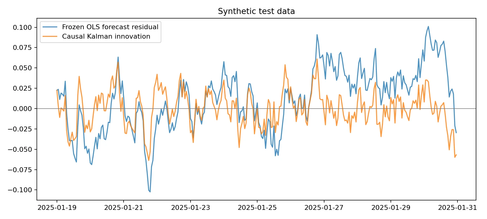
The lines show prediction errors, not profits. A value near zero means that, at that observation, the estimated ETH log price was close to the generated ETH log price. A large deviation means the estimate missed the observed value.
In the supplied deterministic synthetic run (seed 42), the frozen OLS root-mean-square error (RMSE) is about 0.0398 log units, while the causal Kalman conditional-estimate RMSE is about 0.0221 log units. These figures are illustrative experiment results; rerun the packaged script to check them.
What does RMSE actually mean?
RMSE is the square root of the average squared error:
If the typical model errors are smaller, RMSE tends to be smaller. But RMSE does not measure transaction costs, risk, turnover, borrowing fees or the speed at which a deviation reverts. A filter that follows a changing relationship may have low RMSE precisely because it adapts quickly, while providing no stable spread suitable for trading.
Try opening output/forecast.csv. It contains
timestamp, actual,
ols_prediction, kalman_prediction, and
kalman_prior_beta. Pick any row and verify that the Kalman
estimate is based on the prior state, before processing that row’s ETH
observation. This makes the experiment auditable rather than just
visually persuasive.
10. Try the same estimation pipeline with real BTC and ETH candles
The research package also includes fetch_kraken.py, an
optional downloader that requests publicly available
hourly BTC/USD and ETH/USD candles from Kraken. Run:
python -m pip install -r requirements.txt
python fetch_kraken.py --output kraken_btc_eth_logs.csv
python kalman_pairs.py --csv kraken_btc_eth_logs.csv --output output_kraken
The downloader saves a snapshot so subsequent experiments can reuse the same observations. It rejects the final unfinished candle, aligns BTC and ETH to the same UTC timestamps, checks for invalid prices, and computes natural logarithms for the model. The script requires internet access and may fail if the exchange API is unavailable.
Important limitations: Kraken’s OHLC endpoint provides at most 720 recent entries per pair. At an hourly interval this is approximately one month of history, not enough to assess long-run stability or strategy profitability. We have not included fabricated “live market results” in this article. Actual estimates will depend on the date you fetch the candles. See the Kraken OHLC API documentation for current endpoint behavior.
On real data, the model asks a slightly narrower question: can the filter provide more adaptive contemporaneous conditional estimates of ETH’s log price using observed BTC? That is useful for diagnosis. It still does not establish a mean-reverting trade, and it is not a one-hour-ahead forecast of both prices.
11. Turning residuals into trading signals: what is still missing?
You might be tempted to buy ETH whenever it is below the Kalman estimate and sell when it rises above. That is a hypothesis, not a trading strategy yet.
To build a genuine pairs strategy, you need a definition of a significant deviation. One candidate is a standardized innovation:
Here is the surprise and is its predicted variance. A large absolute suggests a deviation bigger than the model typically expects, under its assumptions. But this is not the same as proving that the deviation is likely to reverse: an adaptive model may learn a new relationship instead.
A real backtest must then specify the direction and size of each leg, the signal time and next possible execution time, rebalancing as beta changes, entry/exit thresholds chosen before the final evaluation, transaction fees, spread and slippage, and financing or funding rates. Any short or leveraged position introduces extra operational and liquidation risks.
For perspective: even if a spread seems to offer a gross 0.3% round-trip opportunity, fees and slippage totaling 0.4% would turn that hypothetical opportunity into a net loss before funding costs. These values are illustrative arithmetic, not measured BTC–ETH trading costs. The linked mean-reversion tutorial walks through a fuller, explicit trading-accounting example.
12. Correlation, cointegration, and adaptive regression are different hypotheses
Readers often hear “BTC and ETH move together” and assume they form a cointegrated pair. The terms are not interchangeable:
| Idea | What it asks | What it does not guarantee |
|---|---|---|
| Return correlation | Do short-period price changes tend to move together? | That a price spread stays near equilibrium |
| Cointegration | Do nonstationary series share a stationary linear combination under an appropriate model? | Profitable trading after costs |
| Fixed OLS regression | What static line best fits training observations? | That beta remains constant |
| Kalman dynamic regression | Can a latent relationship be updated sequentially? | Stationarity, cointegration or tradable mean reversion |
In classical Engle–Granger cointegration analysis, the long-run relationship uses a fixed vector of coefficients under its assumptions. If beta changes every hour, ordinary fixed-vector cointegration conclusions cannot be transferred automatically. A Kalman filter can fit two unrelated trending sequences surprisingly well. That is not statistical arbitrage.
13. Four mistakes that make Kalman results look better than they are
Mistake 1: update, then pretend you predicted
Suppose a candle closes at 14:00. You must not update the filter using ETH’s 14:00 close and then claim the updated model was available before that same close. First log the pre-update estimate and innovation; update afterward. If you decide to trade after seeing the close, the backtest must model an execution opportunity that occurs later.
Mistake 2: tune Q and R on the held-out test
Trying 100 settings on the evaluation period and reporting only the winner makes that period part of the model-selection process. Choose parameters on earlier training/validation windows, then reserve a final untouched period to estimate performance.
Mistake 3: interpret forecast RMSE as trading profit
A method can achieve excellent tracking accuracy while adapting away the very spread you hoped to trade. Prediction performance and trading performance are different objectives. Report both separately, and do not insert a pretend equity curve for a model that never simulated positions.
Mistake 4: forget that real trading changes the problem
Missing bars, inconsistent exchange timestamps, short availability, bid/ask spreads, funding fees, liquidity, margin requirements and structural breaks all change the economics. A moving hedge ratio also implies extra turnover. An elegant state-space equation cannot remove those constraints.
14. A more serious evaluation plan
For a publication-quality market study, we would collect a longer immutable dataset, identify several distinct regimes, train on one historical window, choose and using later-but-still-past validation windows, and evaluate on strictly unseen periods. We would repeat with walk-forward splits and compare against several baselines:
- Frozen OLS: coefficients stay fixed after training.
- Rolling OLS: coefficients are re-estimated using only earlier observations in a fixed trailing window.
- Kalman regression: coefficients update sequentially, with noise assumptions fixed before evaluation.
- A naive baseline: a simple persistence or no-change model, to check whether complexity adds genuine value.
We would report errors with uncertainty, residual autocorrelation, parameter stability, number of observations and the behavior of the fitted beta. Only after selecting a separate, fully specified trading rule would we evaluate after-cost P&L, drawdowns and robustness. Where possible, we would publish the data snapshot identifiers and scripts so readers could reproduce the comparisons.
15. What did we actually learn?
We started with a concrete crypto-market question: Has ETH moved unusually far relative to BTC? A regression provides a baseline relationship, but a fixed beta can become stale. A Kalman filter treats that relationship as something that can evolve. It forecasts from its previous estimate, measures the new surprise, and updates the estimate according to uncertainty. Python makes the whole process inspectable.
The key intellectual distinction is estimation versus economic edge. Our synthetic experiment demonstrates adaptive estimation; the optional real-market workflow lets you explore whether the model still behaves sensibly outside a controlled dataset. Neither alone establishes mean reversion or profits. That is not a weakness of the tutorial—it is the correct scientific boundary of the result.
Next steps: work through Mean Reversion Trading in Python to see z-score rules, stationarity tests and an after-cost pairs backtest. Then explore Monte Carlo Methods in Quantitative Finance to practice uncertainty modeling. If you want to check what you actually understood, try the Algonique Quantitative Finance Skill Assessment.
Frequently asked questions
Is a Kalman filter too advanced for beginners? Not if you learn it in the right order. First understand a changing estimate, then the idea of uncertainty, then the equations. The scalar worked example in this tutorial explains the central gain formula before introducing matrices.
What is a dynamic hedge ratio? A regression sensitivity coefficient that changes over time. In a research pairs-trading context, it may also guide the relative size of exposures, but realistic positions require a separately specified execution and rebalancing model.
Why not just use a moving average? A moving average smooths past values. A Kalman filter explicitly models uncertainty in a latent state and noisy observations, and updates its estimates according to both. It is more flexible but also requires defensible assumptions about and .
Does Kalman filtering prove BTC and ETH are cointegrated? No. A dynamic regression and fixed-vector cointegration answer different statistical questions. Adaptation can reduce residual error without establishing a stationary equilibrium.
Can I make money trading the Kalman innovation? Not necessarily. Its sign and size might help define a signal, but profitability depends on whether deviations reliably reverse, risk management, real execution, fees, financing, regime changes and careful out-of-sample validation.
Does the sample code use future information? The filter stores pre-update estimates for each evaluated observation and updates on that observation only afterward. This avoids a common form of same-observation leakage. The code still estimates ETH conditionally on the current known BTC observation, not the future prices of either asset; trading requires an explicit later execution time.
Why are the experiment charts labeled synthetic? We generate the data ourselves to demonstrate the algorithm under known conditions. Labeling this clearly prevents the false impression that the charts show verified historical crypto performance.
References and further learning
- Welch & Bishop — An Introduction to the Kalman Filter. A classic technical introduction to the prediction and update recursions.
- statsmodels — State Space Models. Further reading on Kalman filtering in statistical time-series models.
- scikit-learn — Time Series Split. Why temporal training/evaluation separation matters.
- Kraken — Get OHLC Data. API behavior, including recent-candle limitations and the unfinished final candle.