Quantitative Finance · Practical Research

Mean Reversion Trading in Python: BTC–ETH Pairs Trading, Z-Scores, Cointegration and Backtesting

Can Bitcoin and Ethereum temporarily diverge in a way that a statistically defensible strategy can exploit? Learn the mathematics, test the hypothesis, and build a reproducible Python backtest.

BTC/USD + ETH/USDRegression & cointegrationZ-score signalsAfter-cost backtesting

Research tutorial · No live orders · Synthetic example charts, not real-market returns

Can a trader make money when Bitcoin and Ethereum temporarily move out of sync? In this hands-on quantitative finance tutorial, we will formulate that idea as a statistical hypothesis, derive the mathematics, download real crypto prices, build a Python strategy, and test what survives transaction costs and out-of-sample evaluation.

What you will build: a research-only BTC/USD–ETH/USD pairs-trading backtest with a fitted hedge ratio, Engle–Granger cointegration test, rolling z-scores, stateful entry/exit rules, next-bar execution, explicit trading costs, an out-of-sample equity curve, and exported diagnostic charts. The complete, executable Python program accompanies this article.

Important: this is an educational research experiment, not investment advice or an automated trading bot. It does not claim that BTC and ETH are currently cointegrated or profitable to trade. A result of “no reliable signal” is a meaningful result. The demonstration runs on Kraken's public OHLC endpoint, and the code also offers an explicitly labeled offline synthetic-data mode for testing the pipeline.

1. The real problem: two assets can move together and still drift apart

Bitcoin and Ethereum often respond to broad cryptocurrency-market news, changes in risk appetite, liquidity conditions, and exchange-specific shocks. Their returns can be correlated. A common trading story therefore goes like this:

“If ETH becomes expensive relative to BTC, short ETH and buy BTC. When the relationship normalizes, close both legs.”

That story has three serious problems. First, what counts as expensive? Second, why should the relationship normalize? Third, can the expected normalization cover two legs' trading fees, slippage, and financing costs?

A chart with two similar-looking lines does not answer those questions. Even two statistically independent random walks can look related over a short interval. Regressing one trending price series on another can produce an impressive-looking fit without a stable economic or statistical relationship. We need a stricter framework.

The hypothesis we want to investigate is:

There may exist a linear combination of BTC and ETH log prices whose deviations are substantially more stable than either log-price series individually, and whose deviations sometimes revert quickly enough to support a tradable relative-value strategy.

Notice the careful wording: this is a hypothesis, not an assumption.

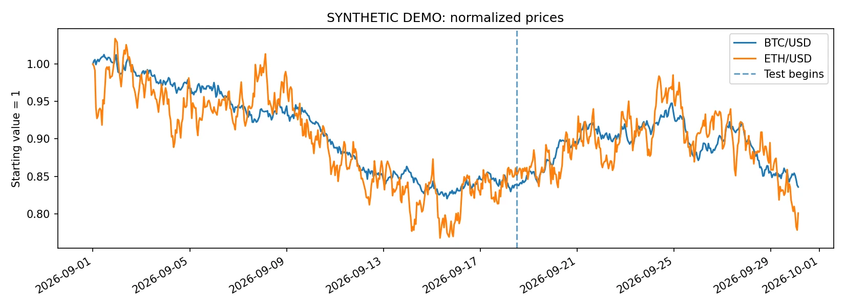
BTC/USD and ETH/USD normalized prices — Synthetic normalized BTC and ETH prices. The dashed line separates the training window from the held-out test window; visual co-movement is not evidence of cointegration.

2. Correlation is not cointegration

Let $P_{B, t}$ denote the BTC/USD price at hour $t$ , and $P_{E, t}$ the ETH/USD price. Define their log prices:

x_{t} = \ln (P_{B, t}), y_{t} = \ln (P_{E, t}) .

Log returns are approximately percentage returns when movements are small:

Δ x_{t} = \ln (P_{B, t}) - \ln (P_{B, t - 1}) \approx \frac{P_{B, t} - P_{B, t - 1}}{P_{B, t - 1}} .

Return correlation measures whether the short-period changes in the two log prices tend to move together:

ρ = \frac{Cov (Δ x_{t}, Δ y_{t})}{σ_{Δ x} σ_{Δ y}} .

A positive $ρ$ says nothing by itself about whether the distance between the two price series is stable. Two assets may move in the same direction on most days while the ratio of their prices trends in one direction for months.

Cointegration asks a stronger question. Suppose $x_{t}$ and $y_{t}$ are each nonstationary, typically modeled as integrated of order one, or $I (1)$ . Are there constants $α$ and $β$ such that

S_{t} = y_{t} - α - β x_{t}

is stationary, $I (0)$ , at least within the regime under study?

If so, the two log prices may share a common stochastic trend while the residual spread fluctuates around a relatively stable equilibrium. This is a statistical relationship, not a promise that the spread will always return to its historical average, and not proof that trading it will make money.

Why use logarithms?

Raw ETH and BTC prices are measured on very different scales. A regression in log prices interprets $β$ approximately as a long-run elasticity: if BTC rises by 1%, the fitted relationship associates it with roughly a $β$ % change in ETH, ignoring short-run residual movements. Log spreads are also convenient for translating their changes into approximate portfolio returns.

There is an important qualification: a log-price spread is a statistical signal, not literally the marked-to-market value of a fixed-share stock portfolio. Our backtest therefore translates it into explicit, dynamically rebalanced dollar exposure weights, rather than pretending that the log spread is a directly tradable security.

3. Estimating the hedge ratio with linear regression

We start with ordinary least squares, fitted only on the training period:

y_{t} = α + β x_{t} + ε_{t} .

With $N$ observations, OLS chooses $\hat{α}$ and $\hat{β}$ to minimize the sum of squared residuals:

min_{α, β} \sum_{t = 1}^{N} (y_{t} - α - β x_{t})^{2} .

For one regressor with an intercept, the familiar closed form is

\hat{β} = \frac{\sum_{t} (x_{t} - \bar{x}) (y_{t} - \bar{y})}{\sum_{t} (x_{t} - \bar{x})^{2}}, \hat{α} = \bar{y} - \hat{β} \bar{x} .

We then freeze these parameters for the test period:

{\hat{S}}_{t} = \ln (P_{E, t}) - \hat{α} - \hat{β} \ln (P_{B, t}) .

Suppose, just for illustration, that the regression gives $\hat{β} = 1.1$ . The strategy would seek to hold ETH and BTC exposures in approximately opposite directions, with a BTC magnitude 1.1 times the ETH exposure. We normalize the gross capital exposure to 1:

w_{E} = \frac{q}{1 + | \hat{β} |}, w_{B} = - \frac{q \hat{β}}{1 + | \hat{β} |},

where $q \in {- 1, 0, + 1}$ is the trading signal. At $\hat{β} = 1.1$ and $q = 1$ , this produces approximately +47.6% ETH and −52.4% BTC gross-notional exposures. In small-return approximation,

r_{p, t} \approx w_{E} r_{E, t} + w_{B} r_{B, t} = \frac{q}{1 + | \hat{β} |} (r_{E, t} - \hat{β} r_{B, t}) .

The first-order change in the log spread is $Δ S_{t} = Δ y_{t} - \hat{β} Δ x_{t}$ . This is why the hedge weights match the signal's mathematics. Because we keep target dollar weights approximately constant, we must rebalance and charge the associated turnover costs; otherwise the P&L calculation would be inconsistent.

A warning about OLS: an apparently high $R^{2}$ in trending financial series can be spurious. Regression is the beginning of the analysis—not its validation.

4. Before trading: are the individual prices I(1)?

Engle–Granger cointegration testing is usually developed for series that are $I (1)$ . We should first examine whether that description is plausible for the two log-price series.

The augmented Dickey–Fuller (ADF) test estimates a regression of the general form

Δ X_{t} = c + γ X_{t - 1} + \sum_{j = 1}^{k} ψ_{j} Δ X_{t - j} + u_{t} .

The null hypothesis is a unit root, roughly $H_{0} : γ = 0$ . A small p-value supports rejecting that null under the specification and assumptions used. A large p-value does not prove a unit root; it means the available evidence was not sufficient to reject it.

For an idealized $I (1)$ candidate, we typically expect the ADF test to fail to reject a unit root for its levels, while rejecting one for its first differences. In actual crypto data, short samples, structural breaks, deterministic trends, and low test power complicate the interpretation.

The project prints all four diagnostics: BTC log-price level, ETH log-price level, and their two first differences. It raises a warning when those checks do not cleanly match the $I (1)$ setup. We do not silently treat every series as integrated.

5. The Engle–Granger cointegration test

The classical two-step Engle–Granger approach first estimates the long-run relationship and then examines whether the fitted residual has a unit root. A critical detail is that ordinary ADF critical values cannot simply be applied to estimated regression residuals as though they were directly observed data: the asymptotic distribution changes when the cointegrating vector is estimated.

Use statsmodels.tsa.stattools.coint, which implements the appropriate Engle–Granger test and its cointegration-specific p-value approximation:

from statsmodels.tsa.stattools import coint

# y_train = log(ETH/USD) and x_train = log(BTC/USD)
t_stat, p_value, critical_values = coint(
    y_train, x_train, trend="c", autolag="aic"
)
print("Engle–Granger p-value:", p_value)

The test's null is no cointegration. A p-value below 0.05 can be evidence against that null in the selected training sample; it is not a declaration that the pair is safe or profitable. The test is also asymmetric in its first-stage regression, sensitive to the chosen sample, and exposed to structural breaks.

BTC and ETH might fail this test. That is a useful finding: a sensible research workflow must allow the hypothesis to fail. The companion program still prints an exploratory backtest for study, but explicitly flags the result if cointegration is not supported in training.

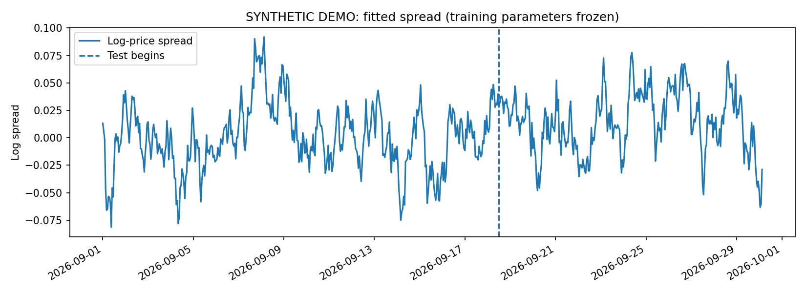
BTC and ETH fitted log-price spread — Synthetic fitted log-price spread with regression parameters estimated on the training sample and held fixed in the test period.

6. Modeling mean reversion: the Ornstein–Uhlenbeck process

The simplest intuitive model for a continuously mean-reverting state variable is an Ornstein–Uhlenbeck (OU) process:

d S_{t} = κ (μ - S_{t}) d t + σ d W_{t},

where:

$S_{t}$ is the spread;
$μ$ is its long-run mean;
$κ > 0$ controls the pull back toward $μ$ ;
$σ$ is the volatility of random shocks;
$W_{t}$ is Brownian motion.

The drift term $κ (μ - S_{t})$ is positive below the mean and negative above the mean. Over a horizon $h$ , the conditional expectation is

E [S_{t + h} ∣ S_{t}] = μ + (S_{t} - μ) e^{- κ h} .

Therefore the expected deviation decays exponentially. The half-life $h_{1 / 2}$ is the time needed for that expected deviation to fall by half:

\frac{1}{2} = e^{- κ h_{1 / 2}} \Rightarrow h_{1 / 2} = \frac{\ln 2}{κ} .

The OU model also gives a conditional variance:

Var (S_{t + h} ∣ S_{t}) = \frac{σ^{2}}{2 κ} (1 - e^{- 2 κ h}) .

This matters because stronger pullback does not eliminate uncertainty. A large negative shock can still move a spread much farther from equilibrium before any correction occurs.

Estimating half-life from hourly data

For equally spaced observations, fit an AR(1) representation to the training residuals:

S_{t} = c + ϕ S_{t - 1} + ϵ_{t} .

Under a discretized OU interpretation with step $Δ = 1$ hour, $ϕ = e^{- κ Δ}$ . Hence

κ = - \frac{\ln (ϕ)}{Δ}, h_{1 / 2} = Δ \frac{\ln (1 / 2)}{\ln (ϕ)} .

The code reports a half-life in hours if $0 < ϕ < 1$ . Otherwise, it reports it as undefined rather than inventing a meaningful value. AR(1) fit on a tiny or nonstationary spread can be misleading, so this is a diagnostic, not a clock that tells us when to sell.

7. From spread to z-score: detecting unusual deviations

The spread is measured in log units, so an absolute threshold like 0.02 is difficult to interpret across assets and regimes. We standardize it by a trailing mean and standard deviation:

Z_{t} = \frac{S_{t} - μ_{t - 1}^{(L)}}{σ_{t - 1}^{(L)}},

where $μ_{t - 1}^{(L)}$ and $σ_{t - 1}^{(L)}$ are computed from the previous $L = 48$ completed hourly spreads—not from future observations and not from a centered moving window.

spread = np.log(data["ETH_close"]) - alpha - beta * np.log(data["BTC_close"])

past_mean = spread.rolling(48, min_periods=48).mean().shift(1)
past_std = spread.rolling(48, min_periods=48).std(ddof=1).shift(1)
z_score = (spread - past_mean) / past_std

Here alpha and beta come from the training regression, and data is the joined hourly dataset. shift(1) makes the rolling reference distribution available before observing the current bar's close. The current close can then be compared with those historical moments to produce a signal for the next bar.

For intuition, $Z_{t} = 2$ means the spread is two trailing sample standard deviations above its trailing mean. It does not guarantee that a Gaussian two-standard-deviation tail probability applies. Crypto returns and residuals often have heavy tails, time-varying volatility, and jumps.

A rolling mean has another limitation: if the relationship breaks and the spread begins trending, the moving average may follow it. A z-score can return toward zero without the original long-run relationship recovering. That is one reason to monitor the underlying spread, the fit's stability, and the behavior of the separate assets—not just the standardized number.

8. Exact strategy rules: entries, exits, and a stop

Our initial thresholds are deliberately simple and fixed in advance:

Condition observed at hourly close	Desired spread position
$2 \leq Z_{t} < 4$ , currently flat	Short ETH / long hedged BTC ( $q = - 1$ )
$- 4 < Z_{t} \leq - 2$ , currently flat	Long ETH / short hedged BTC ( $q = + 1$ )
Existing long-spread trade and $Z_{t} \geq - 0.5$	Close position
Existing short-spread trade and $Z_{t} \leq + 0.5$	Close position
$\| Z_{t} \| \geq 4$	Exit or stay flat (risk stop)
Otherwise	Keep current position

Why two different entry and exit levels? This is hysteresis. If we entered at $Z = 2$ and exited the moment the z-score dipped to 1.99, tiny moves could cause excessive turnover. Requiring a substantial move back toward the center may reduce whipsaw, although this particular parameter choice has not been proven optimal.

Why not automatically enter at $Z = 5$ ? A very large deviation can be a warning that the original relationship has broken. Here $| Z | \geq 4$ is a simple protective rule; it is not a guarantee of a small realized loss, because execution happens later and crypto markets can gap or move rapidly.

Most importantly, thresholds are not optimized on the held-out test sample. Choosing the parameters after seeing which values made money in the test period would contaminate the experiment.

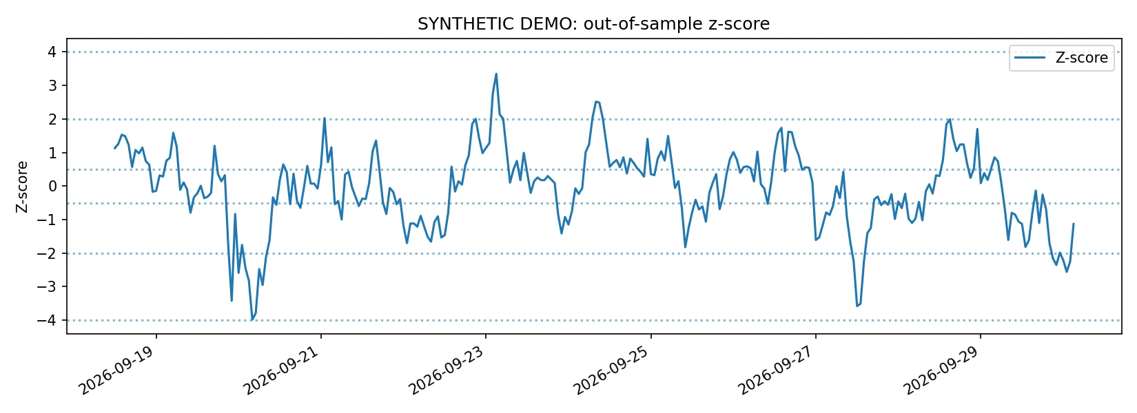
Out-of-sample z-score thresholds — Synthetic out-of-sample z-score. Dotted reference levels show the strategy entry, exit and stop thresholds; signals are computed from past and current completed bars.

9. Real cryptocurrency data: no API key needed

The complete script calls Kraken's public GET /0/public/OHLC endpoint twice: once for XBTUSD (Kraken's BTC symbol) and once for ETHUSD.

import requests

endpoint = "https://api.kraken.com/0/public/OHLC"
response = requests.get(
    endpoint, params={"pair": "XBTUSD", "interval": 60}, timeout=25
)
response.raise_for_status()
payload = response.json()
if payload["error"]:
    raise RuntimeError(payload["error"])
result = payload["result"]
pair_key = next(key for key in result if key != "last")
rows = result[pair_key][:-1]

The final slice [:-1] is essential: Kraken documents that the final OHLC row is the current, unfinished candle. Feeding that changing close price into a historical backtest would pollute the results.

The endpoint returns at most 720 recent candles. On the hourly interval, that gives approximately 30 days of data, not years of reliable history. The script joins the two assets on exact UTC timestamps, validates continuity, saves the downloaded snapshot to CSV, and splits the sample chronologically into approximately 60% training and 40% test.

This is sufficient for demonstrating an honest research workflow, but typically far too short for robust strategy validation, estimating the effect of different market regimes, or confidently annualizing returns. For production-grade research, obtain a longer, immutable historical dataset—for example, Kraken's downloadable OHLCVT archive—and repeat the process on multiple nonoverlapping periods.

No account, exchange key, or live trading permission is used by the program. Real spot-market short positions might require margin, eligible exchange products, borrowing, or derivatives. The backtest models exposures, not executable exchange orders.

10. Backtesting without look-ahead bias

A strategy can appear profitable because of one tiny timing mistake. Suppose the z-score at hourly candle $t$ uses that candle's closing price. It cannot safely be treated as an instruction that was already executed at that same closing price: we only know the final close when the bar has completed.

We use the following timeline:

Close of bar $t$ : observe both closing prices, compute spread and z-score, determine desired state.
Open of bar $t + 1$ : implement the state decided from the previous close.
Between opens $t + 1$ and $t + 2$ : realize the weighted return of the two assets.
At the next open: rebalance the target weights as necessary and charge turnover cost.

In the implementation, the signal is shifted one bar:

test["close_signal"] = signal_states(test["z"])
test["open_state"] = test["close_signal"].shift(1).fillna(0).astype(int)

The script also begins the test flat, even if a training-period bar might otherwise have indicated an entry, and explicitly liquidates at the final observed open to account for the final turnover. That avoids smuggling an unknown pre-test position into the reported result or omitting exit costs.

The actual portfolio P&L

At each open we hold fixed target dollar weights $w_{E, t}$ and $w_{B, t}$ for the next hourly open-to-open interval. Define simple returns

R_{E, t \to t + 1} = \frac{P_{E, open, t + 1}}{P_{E, open, t}} - 1, R_{B, t \to t + 1} = \frac{P_{B, open, t + 1}}{P_{B, open, t}} - 1.

The first-order portfolio gross return is

R_{p, t}^{gross} = w_{E, t} R_{E, t \to t + 1} + w_{B, t} R_{B, t \to t + 1} .

The program charges an illustrative 15 basis points per dollar actually traded (0.0015 times gross traded notional), covering a combined fee/slippage assumption. We charge this on entry, exit, and changes required to rebalance positions whose weights drifted with prices. For instance, opening a full gross-notional position costs approximately 0.15% of the reference portfolio capital, and closing another full notional costs about 0.15%, before any additional rebalancing. That is roughly 0.30% round-trip, not 0.15% for both actions combined.

The model computes the drifted portfolio weights at each opening price, compares them with the next target weights, and charges the absolute difference as turnover:

T_{t} = | w_{E, t} - {\tilde{w}}_{E, t} | + | w_{B, t} - {\tilde{w}}_{B, t} |,

R_{p, t}^{net} = R_{p, t}^{gross} - \frac{15}{10,000} T_{t} .

The tilde denotes weights after price movements but before rebalancing. This accounting is still a simplifying return model: it ignores market impact, changing spread, financing, exchange constraints, liquidation mechanics, and the distinction between gross- and net-capital normalization following a fee. It is far more informative than a backtest with zero costs but is not execution-grade.

Finally, equity compounds net returns:

V_{t} = V_{t - 1} (1 + R_{p, t}^{net}), V_{0} = 1.

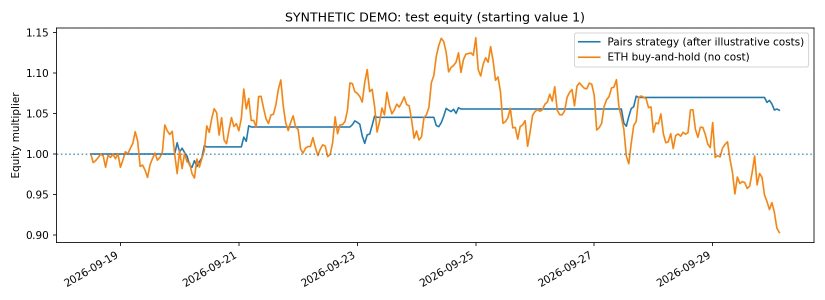
For a benchmark, the script also plots simply buying and holding ETH over the same test interval. This is a visual reference, not a risk-matched performance comparison: a two-leg partially hedged strategy and a directional long-ETH investment have very different exposures.

Strategy equity versus ETH buy-and-hold — Synthetic demonstration only: illustrative after-cost pairs-trading equity compared with unadjusted ETH buy-and-hold, not a real-market performance claim.

11. Run the complete Python experiment

The downloadable research package contains the complete mean_reversion_crypto.py program, requirements.txt, automated tests, and example charts produced only from labeled synthetic data.

Requirements: Python 3.10 or later and an internet connection for real Kraken data. The actual package can be run in a virtual environment:

python3 -m venv .venv
source .venv/bin/activate           # Windows PowerShell: .venv\Scripts\Activate.ps1
python -m pip install -r requirements.txt

# Download actual hourly BTC/USD and ETH/USD candles from Kraken:
python mean_reversion_crypto.py

# Run again against exactly the same saved CSV snapshot:
python mean_reversion_crypto.py

# Ask the endpoint for a fresh snapshot:
python mean_reversion_crypto.py --refresh

# Offline deterministic smoke test using SYNTHETIC prices:
python mean_reversion_crypto.py --demo

# Run the seven automated tests:
python -m pytest -q

The project saves kraken_btc_eth_1h.csv when a real download succeeds. It creates output/real_kraken/ for real-data charts and test rows, or output/synthetic_demo/ for clearly distinguished synthetic experiments. Never present synthetic charts as if they were real market results.

You get four graphs:

btc_eth_prices.png: normalized BTC and ETH close prices with a clear train/test boundary;
spread_train_test.png: the estimated log spread and any shifts in its behavior;
test_zscore_signals.png: out-of-sample z-scores and the relevant threshold levels;
test_equity.png: after-cost strategy equity alongside an unadjusted ETH buy-and-hold reference.

You also get a timestamped backtest_test_rows.csv with spreads, signals, exposures, turnover, costs, and returns. These rows make the experiment inspectable: a reader can audit when a signal was generated and which open-to-open move its position captured.

How to read the output

The console prints training parameters (alpha, beta), an Engle–Granger p-value, the four ADF p-values, an AR(1) persistence estimate and half-life, plus test metrics: total return, maximum drawdown, indicative annualized Sharpe, trade-entry count, time in market, and summed transaction-cost drag.

Do not overinterpret the annualized Sharpe ratio. Multiplying hourly Sharpe by $\sqrt{24 \times 365}$ relies on assumptions about stable return behavior and scaling. A test with only a few hundred bars and potentially highly autocorrelated or non-Gaussian returns gives an unstable annualized number. A high reported Sharpe over two weeks is not evidence that the strategy has a high annual Sharpe in the real world.

We intentionally do not publish invented “real BTC–ETH profits” here. Because prices are fetched at run time, results vary by date and API availability. Run the code, keep the CSV snapshot, record the test interval, and report the actual outcome—even if it is negative or produces almost no trades.

12. When the strategy fails—and what you learn

A losing backtest is not automatically a failure of the tutorial. It can reveal a failed hypothesis. Investigate these failure modes:

High return correlation, no cointegration. The two assets move together but their relative valuation trends, so simple z-score fade trades can systematically lose.

Regime change. A new narrative, protocol event, liquidity shock, or market structure change can break an apparently stable relationship. Fixed regression parameters then stop describing the data.

Small edge, large costs. Even if the spread moves in the expected direction, gross gains may be smaller than the combined entry, rebalancing, and exit expenses.

False confidence from a short backtest. A dozen favorable trades are not enough to infer a robust distribution of future returns. Strategy selection across many pairs or parameter choices also creates multiple-testing and data-snooping problems.

Forced exit does not limit realized loss. A z-score stop does not act instantaneously in the script. It is decided at one close and implemented at the next open; the path between these events can be costly.

Financing and shorting are not free. Synthetic short exposures ignore instrument availability, borrow rates, funding, margin, liquidation thresholds, and counterparty risk. These can dominate expected profits.

Rebalancing is real trading. A portfolio that claims to hold fixed dollar weights must transact as prices move. Trading costs must account for this additional turnover.

The goal of a good quantitative experiment is not to produce an attractive chart. It is to discover which assumptions fail first.

13. Making the model more serious: five next experiments

Our 720-hour dataset is deliberately modest. The natural next project is not “tune the thresholds until the graph is green”; it is to evaluate whether the apparent effect is stable under better research design.

A. Longer and frozen datasets. Obtain multi-year, fixed-snapshot OHLCVT data, keep original timestamps and quote currencies, document missing intervals, and repeat experiments across bull, bear, and sideways regimes. Kraken provides historical OHLCVT download resources in addition to its short rolling API endpoint.

B. Walk-forward fitting. Instead of one 60/40 split, train a model on a fixed historical window, evaluate on the following unseen period, advance time, and refit using only data already available. Keep every evaluated test window out of parameter selection.

C. Structural-break diagnostics. Monitor the training-vs-test hedge ratio, residual mean, residual volatility, rolling stationarity, and the persistence of cointegration. Stop relying on historical relationships that have visibly changed.

D. Alternative statistical models. Compare a rolling hedge ratio, robust regression, error-correction models, and a state-space/Kalman-filter estimate. Dynamic estimates must be updated causally—not using smoothed future information.

E. Real execution modeling. Add bid/ask prices, spread crossing, maker/taker fee schedules, stochastic fills, leverage and margin requirements, funding/borrowing costs, realistic trade sizes, and latency. Run a paper-trading forward test before interpreting any simulation as deployable.

An extension would also use a proper risk-matched benchmark and report confidence intervals, parameter sensitivity, exposure distributions, and performance before and after fees.

14. Frequently asked questions

Is BTC/ETH mean reversion profitable?

Not necessarily. BTC and ETH can be strongly correlated without maintaining a stationary log-price spread, and an apparently mean-reverting relationship may deteriorate. Profitability depends on the sampling period, instrument choice, execution constraints, financing, fees, regime stability, and data quality. A reproducible backtest must measure these factors rather than presume a profitable opportunity.

Is z-score trading the same as statistical arbitrage?

A z-score is merely a normalized signal. Statistical arbitrage usually refers to a broader family of systematically designed relative-value strategies seeking probabilistic rather than risk-free profit. A high z-score alone does not establish cointegration, expected reversal, or a profitable strategy.

Why use cointegration instead of correlation for pairs trading?

Correlation describes contemporaneous comovement, typically of returns. Cointegration studies whether nonstationary level series share a relatively stationary linear combination. That is closer to the long-run equilibrium hypothesis behind pairs trading, although even cointegration does not guarantee short-term predictability or profit.

What does a mean-reversion half-life of six hours mean?

Under a fitted OU/AR(1) model, it means the conditional expected distance from equilibrium decays by half in about six hours. It does not mean every trade closes profitably in six hours or that losses are bounded.

Why does the Python backtest sometimes report no cointegration?

Because BTC and ETH are not guaranteed to form a stable statistical pair in any arbitrary sample. That warning is part of the scientific result, not a Python error. The program still runs an explicitly exploratory diagnostic backtest, but a failed training test should prevent treating its trading signals as validated.

Can this script trade automatically on Kraken?

No. It only downloads public candles and computes research metrics; there are no private account keys, order-placement endpoints, position-sizing safeguards, financing models, or brokerage connectivity. Converting a backtest to a live strategy is a separate engineering and risk-management project.

15. Final lesson: prove the relationship before trading it

Mean reversion sounds simple: buy what is unusually cheap and sell what is unusually expensive. Quantitative finance makes that idea demanding, because cheap, expensive, unusual, and profitable each need a defensible definition.

This case study moves step by step from the economic intuition to a regression-based hedge ratio, cointegration diagnostics, OU half-life, rolling z-scores, causal trade timing, rebalanced portfolio returns, and after-cost out-of-sample evaluation. At every stage we preserve the possibility that the hypothesis is wrong.

That is the larger lesson: a reliable quantitative strategy is not a clever entry rule; it is an evidence chain that survives honest testing.

Test your quantitative finance knowledge: Think you could explain why a stationary spread is different from correlated returns, or identify a look-ahead bug in a backtest? Try the Algonique Quant Skill Assessment to evaluate your understanding of quantitative finance, statistics, and related concepts.

Primary technical references

Kraken REST API: Get OHLC Data — public candles, unfinished last bar, and 720-candle limit.
Kraken: Downloadable Historical OHLCVT Data — longer historical files for research.
statsmodels: Engle–Granger cointegration test (coint) — null hypothesis and cointegration p-values.
statsmodels: Augmented Dickey–Fuller test (adfuller) — test assumptions, lag selection, and unit-root null.

Editorial note: The backtest is intentionally illustrative. The accompanying package has been executed and unit-tested using synthetic offline data; a real-data Kraken execution must be performed on a networked machine before adding any live-market results or real-market chart images to the published page.

From theory to understanding

Do You Understand the Mathematics Behind Quant Trading?

Reading a strategy is one thing. Explaining why it works, recognizing when it fails, and detecting hidden backtest errors requires a deeper level of understanding.

Explore Quant Skill Assessment Understand the assumptions. Test the evidence. Find your knowledge gaps.