Interest Rate Swap Pricing in Python: Yield Curves, Discount Factors and DV01
Learn how banks value an interest rate swap from first principles. We begin with a company’s floating-rate loan, work through a cash-flow example, build a discount curve from market quotes, calculate a fair fixed rate, and measure interest-rate risk. By the end, you can run and test the complete Python pricer yourself.
Level: beginner-friendly, progressing to intermediate quantitative finance
Time to work through: about 35–50 minutes plus optional coding experiments
Tools: Python, NumPy, Matplotlib, pytest
You will build: a five-year, annual-pay, spot-starting single-curve interest rate swap pricer, cash-flow reports, seven explanatory charts, and market-quote DV01 diagnostics.
Model boundary: The rates in this tutorial are deliberately invented: 2.80%, 2.90%, 3.00%, 3.10%, and 3.20% for one- through five-year annual-pay par swaps. They are not current SOFR rates or tradable quotes. Annual accrual factors are set to exactly one year. This teaching model is useful for understanding valuation identities, but does not replace an institutional SOFR swap pricer with actual calendars, daily compounding, clearing rules and collateral conventions.
What problem are we solving?
Imagine a business called Northstar Manufacturing. It has borrowed $100 million for five years at a floating interest rate. Every time market interest rates rise, its borrowing cost may increase. Northstar would prefer predictable financing costs, so it approaches a bank and asks:
“Can we exchange the changing interest rate on our loan for a fixed interest rate?”
That is the motivation for an interest rate swap. The bank and company do not need to exchange the $100 million principal. Instead, on scheduled payment dates, they exchange interest amounts calculated on that notional principal.
The company pays fixed and receives floating under the swap. The floating amount it receives can help offset the floating interest it owes on the loan, assuming the loan and swap reference rates and reset conventions align closely.
| Cash flow | If a year’s floating reference rate is 2% | If it is 5% |
|---|---|---|
| Floating interest owed on $100m loan, excluding spread | −$2,000,000 | −$5,000,000 |
| Floating amount received from swap | +$2,000,000 | +$5,000,000 |
| Fixed amount paid on swap at 3% | −$3,000,000 | −$3,000,000 |
| Combined benchmark-linked amount | −$3,000,000 | −$3,000,000 |
That table ignores loan credit spread, basis differences, fees and imperfect payment-date matching. It establishes the basic idea: the fixed rate replaces the uncertain benchmark-linked amount. The trade is a hedge, not an attempt to predict rates.
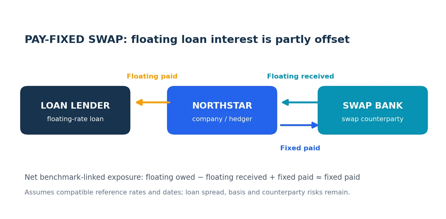
Concept diagram. Northstar pays floating interest to the lender, receives floating from the swap bank, and pays fixed to the bank. The two floating cash flows offset only to the extent that their benchmarks, reset dates and other terms match.
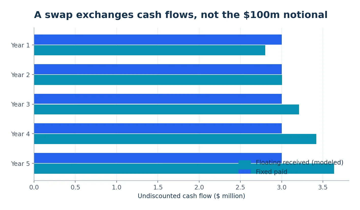
Figure 1. Our Python model creates one payment per year. A fixed-payer swap sends the fixed payments and receives the floating payments. This chart shows amounts at each future payment date, before discounting them to today’s value.
But here is the question that makes this a quantitative-finance problem: what fixed rate should the bank charge? Picking 3% because it sounds reasonable could make one party an immediate economic winner. We need a rate that makes the market value of both sides equal when the contract is agreed.
1. Four ideas to understand before the mathematics
1.1 Notional is not the price of the swap
The notional is the amount on which interest is calculated. In our example, it is $100 million. In a standard interest rate swap, that $100 million is typically not transferred between counterparties. The actual cash flows are calculated as interest on the notional.
If the annual fixed coupon is 3%, then the fixed payment under our deliberately simplified annual accrual convention is:
The final factor of 1 is the accrual fraction: we are modeling exactly one year per coupon. Real schedules use a day-count convention and may have partial periods.
1.2 A floating payment is based on a rate that changes
A floating payment has a similar structure:
where N is notional, αᵢ is the accrual fraction and Lᵢ is the floating rate applicable to period i. For example, $100 million at 4% over a full year produces $4 million of floating interest.
Different swap types define their floating rates differently. Modern U.S. dollar SOFR overnight-indexed swaps typically use a compounded overnight rate over an accrual period. We will first use a mathematically simpler forward rate derived from one curve. We will explicitly return to the real convention later.
1.3 Present value: a dollar tomorrow is not a dollar today
Would you prefer to receive $100 now or $100 in three years? All else equal, most investors prefer it now: today’s money can be invested. Discounting translates future cash flows into present-day amounts.
A discount factor D(t) answers: “How much is $1 paid at time t worth today, under our chosen curve?” If D(3) = 0.9150, then $1 received in three years is worth about $0.9150 today under that curve. A future $3 million payment is worth roughly:
Discount factors depend on maturity. A yield curve is not simply one interest rate applied to every payment.
1.4 Two legs, one net market value
The swap contains two series of payments, called legs. We calculate the value of each leg separately, then subtract:
A positive result means the swap is worth money to the payer of the fixed rate, using this sign convention. A negative result means the payer would, in an idealized mark-to-market settlement, owe value rather than receive it. Neither sign tells us what the company should do with its underlying loan.
2. A yield curve is more than a line on a chart
People often speak of the interest rate as if it were a single number. In reality, financial instruments with different maturities can trade at different interest rates. A one-year swap might have one fixed rate, while a five-year swap has another.
For our exercise, assume the following synthetic par swap quotes. Each is the annual fixed rate that makes a new spot-starting annual-pay swap of that maturity worth zero in our simplified market.
| Maturity | Illustrative par swap quote |
|---|---|
| 1 year | 2.80% |
| 2 years | 2.90% |
| 3 years | 3.00% |
| 4 years | 3.10% |
| 5 years | 3.20% |
Two rates are easy to confuse:
- A par swap rate is the single fixed coupon making all fixed payments balance the floating leg at inception.
- A zero rate is the rate associated with discounting a single payment at one maturity.
These are related but not identical. The five-year swap quote describes five annual coupons, whereas the five-year zero rate describes the present value of one payment five years away.
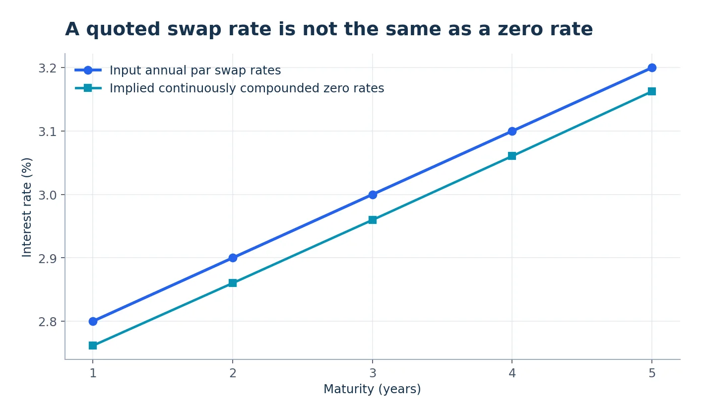
Figure 2. The blue line gives our invented market quotes. The teal line shows continuously compounded zero rates derived from the discount factors. They need not match at each maturity because they summarize different payment patterns.
A pricing system often stores the full curve of discount factors rather than only the quoted par rates. Let’s construct that curve ourselves.
3. Discount factors, explained with one payment
For a simple, one-year payment with an annual rate r, a useful relationship is:
If r = 2.80%, then:
That means $1 received one year from now is worth about 97.28 cents today under this one-year discount rate. It does not mean we should discount every later payment by 0.9727626. A five-year cash flow gets its own discount factor.
Why this formula? If you invest $0.9727626 today at 2.80% for one year, the future value is approximately $1. This is just compound-interest arithmetic run backwards.
For continuously compounded zero rates we instead write:
Here z(t) is the continuously compounded zero rate for maturity t, not the annual-pay par swap quote. The distinction between compounding conventions is important; we do not silently equate a simple rate and a continuously compounded rate.
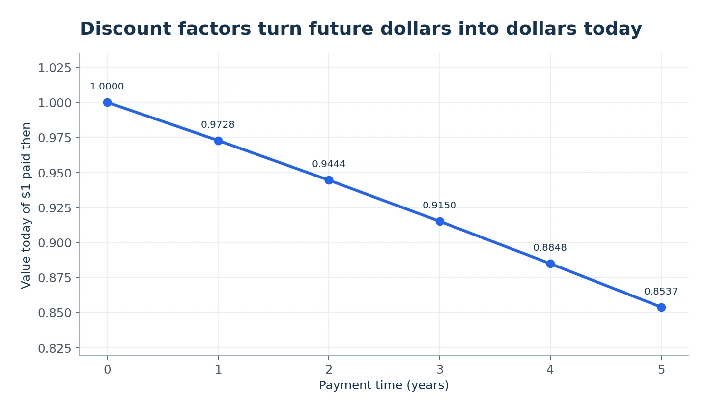
Figure 3. The modeled present value of $1 paid at each maturity. Positive discount rates make these discount factors decrease in this example. With sufficiently negative market rates, discount factors can be greater than one—so decreasing discount factors are not a universal mathematical law.
4. Bootstrapping: build the curve one maturity at a time
Bootstrapping means solving for unknown discount factors sequentially using observable instrument prices or quotes. In this case, the observations are our invented par swap rates, with one new year added at each step.
The useful trick is that once we have solved for D(1), the two-year quote determines D(2). Once D(1) and D(2) are known, the three-year quote determines D(3), and so on.
First year: only one unknown
The one-year par fixed rate K₁ = 2.80% must satisfy:
Rearranging gives exactly the one-year formula above: D(1) = 1/(1 + K₁).
Second year: now we use two discount factors
The two-year par swap has two fixed coupons: one at year 1 and one at year 2. Under our single-curve assumptions, the floating leg has present value 1 − D(2) per dollar notional. So:
Move the D(2) terms together:
We already know D(1) = 0.9727626 and K₂ = 0.029. Therefore:
You can now do the two-year swap valuation yourself: the present value of its fixed leg equals 2.90% × [D(1) + D(2)] × notional, exactly the value of its floating leg.
Third through fifth years: same idea
At year n the par swap rate is Kₙ and the preceding discount factors have already been calculated:
Solve for the single remaining unknown:
This formula is not the universal bootstrap formula for every rates instrument. It works here because coupon dates coincide exactly with the annual curve nodes, every accrual fraction is 1, swaps start today, all floating periods use the same curve, and there are no schedule complications. Real curve construction requires instrument-specific valuation equations and often numerical root finding.
Our full example produces:
| Year | Par swap quote | Solved D(year) |
|---|---|---|
| 1 | 2.80% | 0.9727626 |
| 2 | 2.90% | 0.9444022 |
| 3 | 3.00% | 0.9150340 |
| 4 | 3.10% | 0.8847738 |
| 5 | 3.20% | 0.8537373 |
The first Python building block
import numpy as np

quotes = np.array([0.028, 0.029, 0.030, 0.031, 0.032])

discounts = [1.0]                    # D(0) = 1
for fixed_rate in quotes:
    prior_coupons_pv = sum(discounts[1:])
    next_df = (1 - fixed_rate * prior_coupons_pv) / (1 + fixed_rate)
    discounts.append(next_df)

print(np.round(discounts, 7))
# [1.        0.9727626 0.9444022 0.915034  0.8847738 0.8537373]
It is deliberately short so you can see the mathematics in the code. The downloadable project contains a fuller version with input checks and nine automated tests.
5. Where do the future floating rates come from?
We have not yet specified any future floating coupons. That’s the next puzzle: How do we value floating payments before we know the rate that will actually prevail?
The curve tells us the forward rates implied by its discount factors. In this annual teaching model, the one-year forward rate for the period from year i−1 to year i is:
More generally, with an accrual fraction αᵢ rather than exactly one year:
Here is the intuition. Suppose you could invest for two years, or invest for one year and then roll into a second one-year investment. If both strategies are priced consistently, the implied one-year rate for the second year is determined by the ratio of the discount factors for years 1 and 2.
Using our curve:
This is a market-implied forward rate, not a prediction guaranteed to be realized. Its purpose here is to make the pricing equations consistent.
| Floating period | Implied annual forward | Floating payment on $100m |
|---|---|---|
| Year 1 | 2.8000% | $2.800m |
| Year 2 | 3.0030% | $3.003m |
| Year 3 | 3.2095% | $3.210m |
| Year 4 | 3.4201% | $3.420m |
| Year 5 | 3.6354% | $3.635m |
The forward rates are different each year—even though the swap will use one fixed rate for all five years. That is exactly why we need present values to compare the two legs.
6. Pricing the fixed leg, one coupon at a time
The value of a fixed interest payment at time i is:
The fixed leg is the sum of those present values:
For our five annual payments, αᵢ = 1. Define the swap annuity (also called the fixed-leg level) as:
This is not an annuity that deposits money into your bank account; it is simply the sum of coupon discount factors with accrual weights. If the previously agreed fixed rate is K = 3.00%:
The undiscounted total would have been $15 million (five payments of $3 million). The present value is lower, because later dollars are discounted.
7. Pricing the floating leg — and a surprisingly useful identity
If every floating payment in the simplified model uses the forward rate from the same curve we use for discounting:
Substitute the forward-rate formula with αᵢ = 1:
Now look at what happens when we add the payment values:
All the middle terms cancel, a phenomenon called a telescoping sum. Thus for this spot-starting, single-curve structure:
Numerically:
This is an extremely useful result for understanding swaps. Do not assume it automatically applies to arbitrary floating legs. It changes when discounting and projection curves differ, when accrual or reset conventions differ from our setup, or when already-fixed coupons are involved.
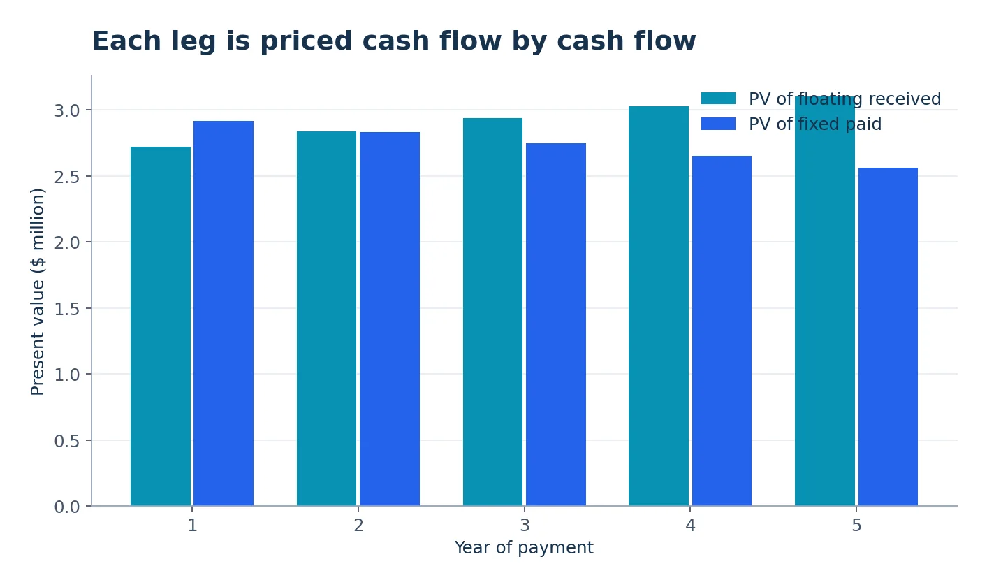
Figure 4. The bars show the discounted value of each fixed and floating cash flow. The blue and teal totals are the two legs’ present values; the difference is the current value of the previously agreed swap.
8. What is the fair fixed swap rate?
A brand-new, at-market swap is normally quoted with a fixed rate making its present value approximately zero at initiation, ignoring bid/ask, fees, credit valuation adjustments and other deal terms.
To find that rate, make the two legs equal:
The notional cancels and we obtain:
Insert our five discount factors:
The five-year market quote we started with was 3.20%, so the exact agreement between the implied rate and the input quote is not a coincidence. Bootstrapping must reprice the original calibration instruments. If it cannot, the curve-building code is wrong or the assumptions do not match the instruments.
But what if the swap was signed earlier at 3%?
Suppose Northstar locked in a 3.00% fixed rate when the swap was first arranged. Today, we observe our example market curve with a new five-year par rate of 3.20%. To keep the illustration consistent, imagine the old contract still has five future annual payments remaining and its schedule matches the new spot-starting model. We are comparing two coupon levels against the same remaining cash-flow schedule, not pretending a partially seasoned historical trade restarts today.
The payer-fixed swap’s present value is:
Another helpful way to write it is:
Here 0.20 percentage points, or 20 basis points, separates the current market par rate from the old contractual coupon. The value is approximately $100m × 4.57071 × 0.002 = $914,142. This is a mark-to-market estimate, not an immediate cash payment to the company and not a measure of its loan’s entire economic value.
notional = 100_000_000
contract_fixed = 0.0300
annuity = sum(discounts[1:])

float_pv = notional * (1 - discounts[-1])
fixed_pv = notional * contract_fixed * annuity
swap_pv = float_pv - fixed_pv
par_rate = (1 - discounts[-1]) / annuity

print(f"Par rate: {par_rate:.2%}")   # 3.20%
print(f"Swap PV: ${swap_pv:,.0f}")  # $914,142
Quick understanding check
If the contractual fixed rate were 3.40%, while the curve still implied a fair rate of 3.20%, would the same fixed payer benefit or lose? The answer is lose, because it would be paying a higher fixed coupon than a new market participant would pay for the same remaining cash flows. The payer-side value would be negative.
9. A basis point sounds tiny. On $100 million, it is not.
Traders and risk managers often discuss rate changes in basis points:
| Change | Decimal change | Percentage-point change |
|---|---|---|
| 1 bp | 0.0001 | 0.01 percentage points |
| 10 bp | 0.0010 | 0.10 percentage points |
| 100 bp | 0.0100 | 1.00 percentage point |
A five-year interest rate swap is sensitive to interest rate movements because a change in the market curve changes the market value of all the remaining payments.
To measure this, we need to be precise about what exactly moves. In the accompanying program, we shift all five input annual par swap quotes up by one basis point, rebuild the discount curve, and revalue the unchanged contractual fixed coupon. We also do the same with a one-basis-point decrease.
That is market-quote curve risk for our specified calibration setup. It is not the same as changing only the discount rate while leaving floating forwards fixed, and it is different from the present value of one basis point on the fixed coupon itself.
DV01 by finite differences
Let V(q) be the swap market value after calibrating to a vector of quotes q. Let h = 0.0001 represent one basis point. A symmetric difference estimates the signed change for a +1bp parallel quote shift:
The numerical derivative would divide this difference by 2h. Here we are instead reporting the dollar change per one-basis-point move, so the formula above already includes the bump size.
For our $100 million, 3%-fixed-payer example:
| Calculation | Result |
|---|---|
| Current swap present value | +$914,142 |
| Value increase after exactly +1bp parallel quote move | approximately +$45,433 |
| Symmetric signed DV01 | approximately +$45,446 per bp |
Why is the fixed-payer DV01 positive? If market rates rise, paying the old 3% rate becomes more advantageous relative to entering a comparable new swap. The positive value is not universal: reverse the trade direction and the sign reverses. Also, industry reports differ in naming and sign conventions—always inspect the risk report’s definition rather than assuming all DV01 labels mean exactly the same thing.
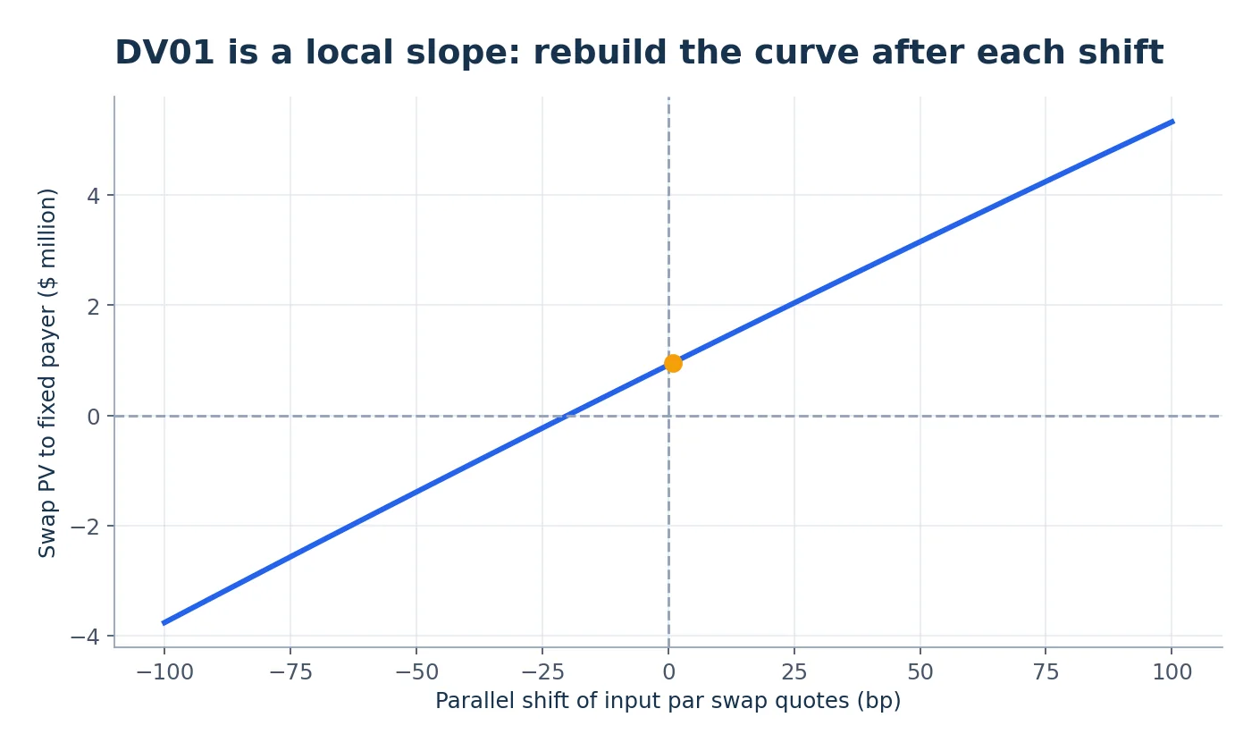
Figure 5. Each point is produced by rebuilding the curve after a parallel shift of the input market swap quotes. DV01 describes the local sensitivity near a zero-basis-point shift; over a much larger change, curvature means a linear DV01 approximation need not be exact.
The actual Python risk calculation
ONE_BP = 0.0001
quotes = np.array([0.028, 0.029, 0.030, 0.031, 0.032])

def pv_for_quotes(market_quotes):
    d = bootstrap_discount_factors(market_quotes)
    return receive_float_pay_fixed_pv(d, 100_000_000, 0.03)

pv_up = pv_for_quotes(quotes + ONE_BP)
pv_down = pv_for_quotes(quotes - ONE_BP)
signed_dv01 = (pv_up - pv_down) / 2
print(f"Signed market-quote DV01: ${signed_dv01:,.2f}")
The final three functions are provided in the downloadable complete Python module. Crucially, we do not change the previously agreed 3% coupon when the market changes. Otherwise we would be comparing different swaps rather than valuing the same contract through time.
10. Key-rate DV01: which part of the curve matters?
An entire curve rarely shifts perfectly in parallel. Perhaps one-year rates rise while five-year rates fall. Banks therefore inspect bucketed sensitivity, also called key-rate risk in this context.
To produce a simple key-rate calculation, we bump only one input par quote at a time by ±1bp, rebuild the curve, and calculate the central finite difference in the trade’s present value. Repeat for each quote maturity.
This exposes how our particular five-year trade responds to small changes in each calibration quote. It is not a universal claim that shorter-dated rates have no effect: the answer depends on the curve parameterization, contract cash flows, chosen instruments, and any interpolation used.
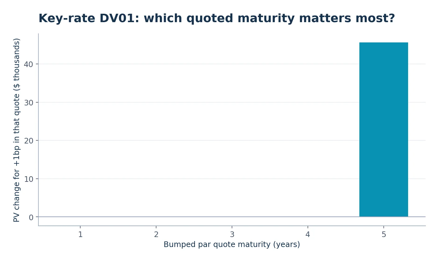
Figure 6. An illustrative quote-bucket risk profile. A five-year instrument in this simple no-interpolation calibration has much of its direct sensitivity concentrated in the five-year par quote. A production trading book may have far more complex key-rate exposure.
An important programming check: the sum of the individual key-rate finite-difference sensitivities should be close to the sensitivity to a small parallel shift. For sufficiently small bumps, both are approximations to the same first-order directional derivative. The tests supplied with the project check that relationship.
11. Run the complete Python project
If you know just enough Python to run a script, you can reproduce all the results. You do not need an exchange account, banking data subscription or API key, because every interest rate used here is explicitly included in the program.
Download the accompanying ZIP from the top of this article. Inside you will find swap_pricing.py, requirements.txt, tests and an explanation of the inputs.
# From the unzipped research/ directory
python3 -m venv .venv
source .venv/bin/activate       # Windows PowerShell: .venv\Scripts\Activate.ps1
python -m pip install -r requirements.txt

python swap_pricing.py --output output
python -m pytest -q
The script produces seven plots and two auditable tables:
| Output | What it shows |
|---|---|
irs-hedge-flow.png |
Who pays fixed and floating in the loan hedge |
irs-leg-cashflows.png |
Floating versus fixed cash flows by year |
irs-par-vs-zero-curve.png |
Quoted swap rates versus derived zero rates |
irs-discount-factors.png |
Present value of $1 across maturities |
irs-leg-present-values.png |
Each payment’s contribution to swap PV |
irs-dv01-scenarios.png |
Swap PV under parallel quote shifts |
irs-key-rate-dv01.png |
DV01 when one market quote changes |
cashflows.csv |
Rates, future payments, discount factors and PVs |
key_rate_dv01.csv |
Signed sensitivities by market-quote tenor |
Reproducibility note: No live market data is requested, and the examples are not a forecast. The program’s formulas and test output describe this carefully specified toy market. If you change the input quote vector, the figures and reported values change accordingly.
Three experiments that will teach you more than memorizing formulas
Experiment A — make the entire curve flat. Change all five par quotes to 3%. What happens to the annual forwards and five-year par rate? You should find that a flat par curve implies a flat annual forward rate in this annual one-curve setup. Ask yourself whether the same statement survives when payment schedules and compounding conventions change.
Experiment B — change only the contractual fixed coupon. Keep market quotes unchanged and try 2.50%, 3.00%, 3.20% and 3.50%. The market curve is the same; only the contract changes. Does swap PV move linearly with the contractual coupon? Yes, because the fixed-leg annuity is fixed when the curve is fixed.
Experiment C — change the notional. Double it from $100 million to $200 million. What happens to PV and DV01? In this deterministic linear swap model, both double. The market’s interest rates and the discount factors do not depend on this notional in the example.
12. How the toy pricer relates to a real SOFR interest rate swap
This section matters because a code example can be mathematically correct while still not implementing the contract that a bank trades.
Overnight compounding instead of one guessed annual floating rate
SOFR, published by the Federal Reserve Bank of New York, is a measure of overnight Treasury-secured borrowing costs. A standard U.S. dollar SOFR overnight-indexed swap (OIS) floating leg often uses business-day-compounded overnight SOFR, not a single annual forecast applied directly to the whole year. The New York Fed documents SOFR, and CME explains overnight compounding conventions.
If a floating accrual period contains daily rates rⱼ and actual/360 accrual fractions δⱼ, a simplified compounded growth factor is:
The relevant business-day schedules, weekend and holiday accrual rules, observation lags, and payment dates are part of the instrument definition. Do not substitute the toy annual-forward payments into a contract with actual compounded SOFR and expect matching cash flows.
A real floating-rate corporate loan may not hedge perfectly
If a company’s loan resets to one reference rate while the swap receives a different rate or has different dates, some uncertainty remains: basis risk. A loan also typically includes a borrower-specific credit spread. The swap hedges the benchmark-linked component, not automatically the entire borrowing cost.
A real valuation uses calendars and explicit conventions
Professional implementations account for day counts, holiday calendars, payment and reset dates, stub periods, settlement lags, known coupons, interpolation, curve extrapolation assumptions, and counterparty/clearing terms. Once an original swap has partially matured, you must use its remaining cash flows and known fixings, not price it as an entirely fresh five-year contract.
Modern curve setups may separate forecasting and discounting
A common modern framework can involve different curves for forecasting future floating coupons and discounting their payments. OpenGamma Strata, for example, explicitly provides separate discounting and forward-curve identifiers and production swap pricing facilities. In a multi-curve model:
and therefore:
Notice the crucial difference: you cannot replace the numerator by 1 − D(T) in a general multi-curve model. We kept projection and discounting on the same curve earlier so you could understand the arithmetic, not because it is a universal market rule.
For production curve construction, teams may calibrate multiple curves to deposits, futures, OIS swaps and other instruments, with instrument-specific equations and solver-based calibration. OpenGamma’s curve calibrator is a useful reference implementation of this more general concept.
13. Common mistakes in interest rate swap pricing
Mistake 1: Treating the par swap rate as a zero rate. A five-year par swap’s fixed coupon weights several cash flows. A five-year zero rate prices one payment. The two curves need not be identical.
Mistake 2: Forgetting the accrual fraction. A rate of 4% does not generate a 4% payment for a three-month period. Day-count conventions determine the accrual amount; our α=1 assumption is a teaching simplification.
Mistake 3: Forgetting the sign convention. Receive-fixed and pay-fixed swaps have opposite sensitivities. Label all outputs from a clearly identified point of view.
Mistake 4: Using the wrong curve for the wrong task. A future floating coupon may be projected from one curve but discounted with another. The identity PVfloating = N(1 − D(T)) is conditional on special assumptions.
Mistake 5: Computing DV01 without defining the shock. Shifting only discount zero rates while freezing forward coupons is not the same risk calculation as shocking the quotes that calibrate both. Even two legitimate DV01 reports can differ if they are measuring different risk definitions.
Mistake 6: Valuing an old swap as if it starts today. Payment dates, previous resets and accrued interest matter. An old fixed coupon can be compared with a newly calibrated curve, but only over the actual remaining schedule.
Mistake 7: Calling model PV the cash that will actually settle. A swap mark-to-market is an estimate of economic value; contractual cash flows, collateral, close-out amounts and funding are separate concepts.
14. Where to take this project next
A natural second-level tutorial would build a realistic SOFR OIS curve, using market conventions for overnight compounding, a calendar, nonuniform accrual factors and curve nodes at irregular maturities. Later you could add separate projection and discount curves, a full portfolio of swaps, key-rate hedging, and valuation adjustments such as CVA/DVA where appropriate.
It is also useful to compare our outputs with a trusted pricing library. OpenGamma Strata exposes swap present value, par rate, PV01 and bucketed risk calculations. That sort of independent benchmark is much more valuable than merely checking that your own chart looks plausible.
The most important lesson: interest rate swap pricing is not about memorizing one elegant formula. It is about understanding which payments happen, when they happen, what curve determines each amount, what discounts those amounts to today, and what assumptions lie behind the reported risk.
Frequently asked questions
What is an interest rate swap in simple terms?
An interest rate swap is a contract in which two parties exchange streams of interest payments, commonly one fixed and one floating, based on an agreed notional. The notional typically serves as a calculation reference rather than a principal exchange.
How do you calculate the fair fixed rate of an interest rate swap?
Discount the expected floating leg and divide by the fixed leg’s accrual-weighted discount-factor sum, times notional as appropriate. In our single-curve annual model, this simplifies to (1 − D(T)) / Σ D(i). Actual products require their own conventions and schedule.
What is the difference between a swap curve and a zero-coupon yield curve?
A par swap curve contains fixed coupons that make whole swap contracts worth zero at inception. A zero curve contains rates that discount individual payments. A calibration process converts observable instruments into curves suitable for valuation.
What is DV01 and is it always positive?
DV01 expresses how present value responds to a one-basis-point change in a specified rate or curve risk factor. Its sign depends on trade direction and reporting convention. Here we use the signed change for a +1bp move in calibrated market swap quotes, so a pay-fixed position has positive DV01 in the example.
Is a five-year swap worth $100 million if its notional is $100 million?
No. Notional is a reference amount used for calculating interest payments. A new fair swap may have a market value close to zero even on a very large notional.
Can I use the supplied Python script to price a live SOFR swap?
Not as-is. It intentionally assumes annual coupon dates, one curve, synthetic par quotes and no real contract-specific schedules. It is an educational research program, not a live market execution or bank-grade valuation engine.
Can interest rate swaps remove all risk from a floating-rate loan?
No. The hedge can offset some benchmark-rate exposure, but differences in indices, payment schedules, credit spreads, counterparty credit, collateral and funding can leave meaningful risks.
References and further reading
- Federal Reserve Bank of New York — SOFR reference rate: what SOFR measures and how it is published.
- CME Group — Understanding SOFR Futures: daily compounded SOFR conventions and relation to overnight indexed swaps.
- OpenGamma Strata — Swap product pricer: present value, par rate and sensitivities.
- OpenGamma Strata — Swap trade calculations: PV01 measures, including calibrated and market-quote views.
- OpenGamma Strata — Rates market data lookup: separate forward and discount curves.
- OpenGamma Strata — Curve calibrator: how instrument quotes feed calibrated term structures.
Explore more on Algonique: Black–Scholes explained · Monte Carlo option pricing in Python · Quantitative Finance Skill Assessment
Educational content and reproducible toy-market research. Not investment, pricing, hedging or trading advice for a real transaction.