Monte Carlo Option Pricing in Python: Black–Scholes, Confidence Intervals, and Variance Reduction
A beginner-friendly, hands-on guide to understanding options, simulating prices, and checking whether a numerical answer is trustworthy.
Imagine that a stock costs $100 today. You have the right—but not the obligation—to buy it for $100 one year from now. If the stock rises to $130, that right is valuable. If it falls to $80, you can simply choose not to buy. How much should you pay today for this right?
That is an option-pricing problem. Instead of guessing one future stock price, we will explore thousands of possible future outcomes with Python, calculate the option’s payoff in each one, and estimate an average under a specific mathematical model. This procedure is called Monte Carlo simulation. We will also learn why the average must be discounted, why we use a risk-neutral distribution, how uncertain our numerical estimate is, and how to make it more accurate without simply throwing millions of extra random numbers at it.
You do not need to know stochastic calculus before reading this guide. We begin with dollar amounts and a tiny example you can work out by hand. Only after that do we introduce Black–Scholes, geometric Brownian motion, the mathematical estimator, and two widely used variance-reduction methods. Every important equation is translated into plain language and tied to Python.
What you will build: a reproducible European call option-pricing lab using NumPy and Matplotlib. It calculates a Black–Scholes benchmark, compares plain Monte Carlo with antithetic variates and a control variate, reports approximate 95% confidence intervals, and produces explanatory charts. All prices and results in this tutorial are model simulations with assumed parameters, not actual option-market quotes or investment recommendations.
Related reading: Black–Scholes Model Explained, Monte Carlo Methods in Quantitative Finance, and the Quantitative Finance Skill Assessment.
1. First understand the financial product: what is a call option?
A European call option gives its buyer the right to purchase an asset at a predetermined strike price on a particular expiration date. European here means exercise occurs at expiration; it does not describe where the option trades.
Let’s assign meanings to the numbers:
- The stock price today is $100, written as .
- The strike price is $100, written as .
- The option expires in one year, written as .
- The unknown stock price at expiration is .
At expiration, compare with . If the stock is $130, you can buy for $100 and receive an asset worth $130: your payoff is $30. If the stock is $80, exercising would be silly, so your payoff is $0.
| Stock at expiration | Right to buy for $100 | Call payoff |
|---|---|---|
| $80 | Not useful | $0 |
| $95 | Not useful | $0 |
| $100 | Break-even exercise value | $0 |
| $110 | Buy an asset worth $110 for $100 | $10 |
| $130 | Buy an asset worth $130 for $100 | $30 |
A single expression summarizes the table:
Read max as “take whichever is
greater.” The floor at zero matters because the option holder
is not required to exercise. Payoff is not profit: if
you paid $9 for the option today, a $10 expiration payoff gives only $1
of undiscounted net cash gain before fees. Our task is to estimate the
option’s model value today, not an investor’s future
profit.
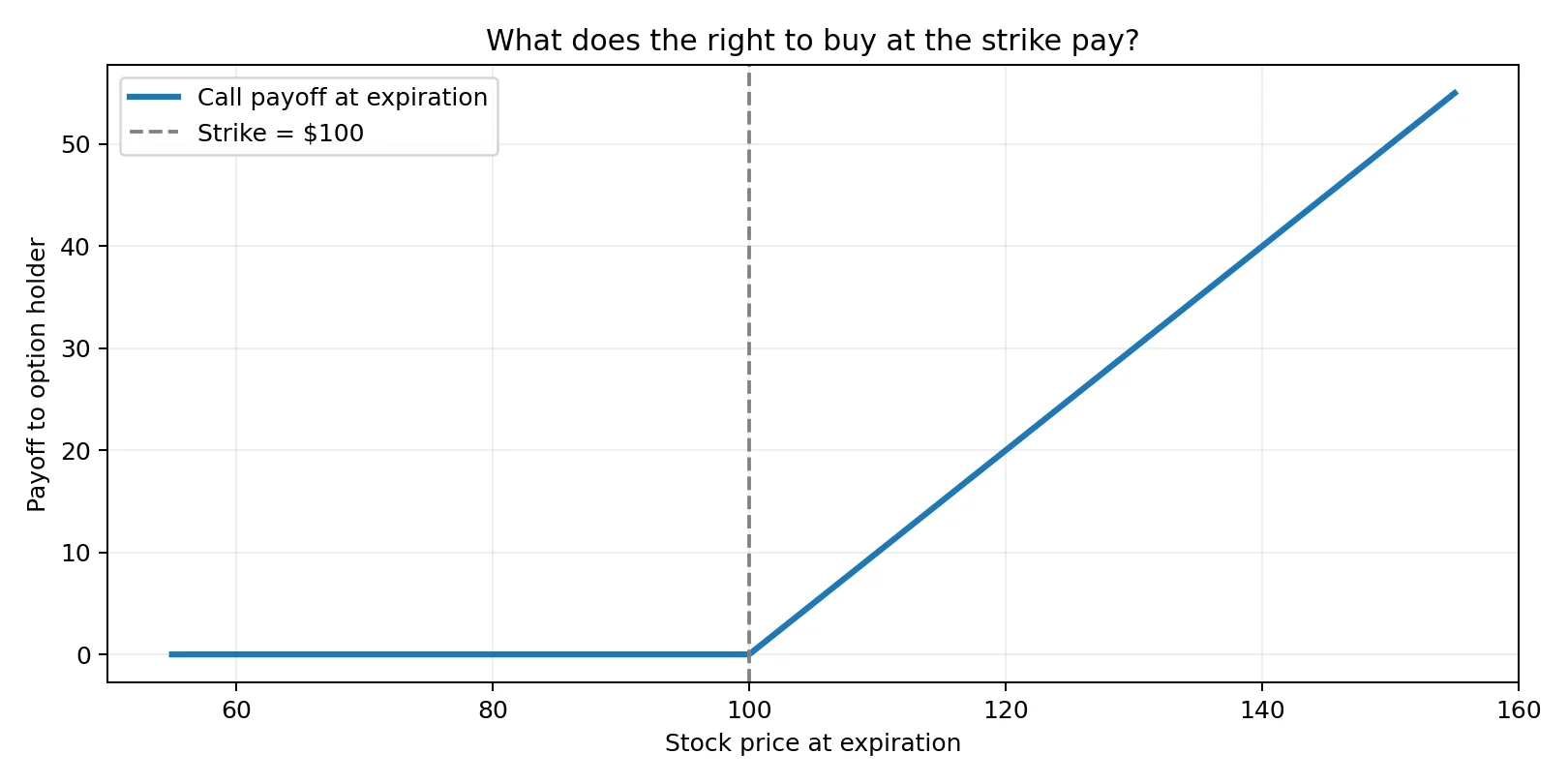
The payoff chart is a deterministic illustration of the contract. It is not a price forecast.
2. Why does pricing an option require thinking about many futures?
No one knows the stock price next year. If we tried to value the call based on a single prediction—“the stock will be $115”—we would ignore uncertainty, even though uncertainty is exactly what makes optionality valuable.
Consider a toy world with only three possible outcomes, all given equal weights:
| Hypothetical final stock price | Call payoff |
|---|---|
| $80 | $0 |
| $100 | $0 |
| $130 | $30 |
The simple average payoff is . At a continuously compounded annual rate of 3%, the corresponding discounted amount is .
Important qualification: these three probabilities were made up for illustration. Their discounted average is not automatically an arbitrage-free option price. Real model pricing requires probabilities consistent with the traded stock and discounting assumptions. We introduce that consistency through the risk-neutral model below.
Now imagine a richer world: instead of three possible prices, generate 10,000 or 100,000 possible final prices using a probability distribution. That is the central Monte Carlo idea:
- Describe mathematically how future prices could be distributed.
- Randomly draw many possible prices from that model.
- Calculate the call payoff for each possible price.
- Average the payoffs and discount to today’s value.
- Measure how much numerical uncertainty remains in this average.
The simulation produces a range of possible outcomes, not a claim about which future will occur.
3. The five inputs: stock, strike, time, interest rate, volatility
Before using an equation, understand every input. We will keep the same illustrative values throughout the article:
| Symbol | Meaning | Our example |
|---|---|---|
| Current stock price | $100 | |
| Option strike price | $100 | |
| Time until expiration, measured in years | 1 | |
| Continuously compounded annual risk-free rate in the model | 3% = 0.03 | |
| Annualized stock-price volatility in the model | 20% = 0.20 |
Volatility is not the expected return. In this model it controls how widely possible price outcomes spread out. With higher volatility, a call has more opportunities to finish substantially above the strike, while losses to the buyer remain limited to the option premium. This is why options can become more valuable when volatility rises.
Interest rate enters differently: it is used for the no-arbitrage pricing distribution and for discounting future cash flows. It is not a confident forecast that the stock will literally earn exactly 3% over the year.
Time is in years. For roughly three months we would use ; for six months, . We assume no dividends, constant volatility and rate, frictionless trading, and the idealized Black–Scholes model. These simplifications help us study the numerical method; they do not describe all real markets.
4. What does “risk-neutral” actually mean?
This is usually the part where tutorials suddenly become mathematical. The intuition is simpler than it first looks.
Suppose two investors disagree about the stock’s likely return: one predicts 5% and another 15%. If a traded European call could have two unrelated no-arbitrage prices solely because of their personal forecasts, there would be an inconsistency. Under the Black–Scholes assumptions, we can price the option instead by working with a special probability measure often denoted .
Under this risk-neutral measure, the stock’s modeled expected growth rate is the risk-free rate (for a non-dividend-paying stock), and we discount the option’s future payoff using the same rate. That combination is justified by the model’s replicating-portfolio/no-arbitrage argument. It does not mean real investors are risk-neutral, and is not necessarily the real-world distribution of future prices.
The conceptual pricing equation is:
Read it from right to left:
- is what the contract pays at expiration.
- means average over the modeled risk-neutral outcomes.
- moves that expected future amount back to today’s value.
- is the resulting today’s model price.
The symbol
is the natural exponential base (about 2.718). Python computes the
discount factor with np.exp(-r * T).
5. How do we generate plausible future stock prices?
We now need a model that turns random numbers into positive future prices. The classical Black–Scholes assumption uses geometric Brownian motion, abbreviated GBM. Think of it as a model with a steady systematic component plus unpredictable random fluctuations, both acting proportionally to the current stock price.
Under the risk-neutral measure, GBM is written:
Don’t worry if the differential notation is new. Its pieces mean:
- : current stock price at time .
- : small deterministic drift in the risk-neutral model.
- : random movement, scaled by volatility.
- : Brownian motion, a mathematical model of accumulated random shocks.
For our European option, we do not even need to simulate every second of the stock’s path. There is an exact formula for the terminal stock price after years:
Here
is a standard normal random variable: values near zero
occur most frequently, while large positive and negative values are
rarer. A new draw of
creates a new possible final stock price.
np.random.default_rng(...).standard_normal(...) supplies
such draws in Python.
Why is there a mysterious term?
Because we model a lognormal terminal stock price, the average of the exponential is not simply the exponential of the average. The correction is the Itô correction that makes the model’s expected terminal price satisfy:
This identity matters. After discounting the terminal stock, the expected value is the starting price: . We will use that identity later to make Monte Carlo much more precise.
For advanced readers: applying Itô’s lemma to yields . Integrating over and using produces the exact terminal formula above. Beginners can use the formula without first mastering stochastic calculus.
6. The first Python experiment: simulate just ten possible futures
Before we write a complete research program, make the simulation
tangible. Create a file named first_ten.py:
import numpy as np

S0 = 100.0       # stock price today
K = 100.0        # strike price
T = 1.0          # one year
r = 0.03         # 3% annual risk-free rate
sigma = 0.20     # 20% annual volatility

rng = np.random.default_rng(42)
z = rng.standard_normal(10)

terminal_prices = S0 * np.exp(
    (r - 0.5 * sigma**2) * T + sigma * np.sqrt(T) * z
)
payoffs = np.maximum(terminal_prices - K, 0.0)
discounted_payoffs = np.exp(-r * T) * payoffs

for index, (stock, payoff) in enumerate(zip(terminal_prices, payoffs), 1):
    print(f"Scenario {index:2d}: stock=${stock:7.2f}; call payoff=${payoff:6.2f}")

print("Estimated option price:", discounted_payoffs.mean())
Every line has an understandable role: z contains ten
random shocks; terminal_prices converts shocks to final
stock values; np.maximum implements the contractual payoff;
and .mean() estimates the discounted expected payoff.
Do not trust the answer from just ten simulations. Run the program with a different seed and it may give a noticeably different price. That instability is not a bug—it demonstrates sampling error. Now we need more draws and a way to quantify the remaining uncertainty.
7. From ten simulations to 100,000: the Monte Carlo estimator
Suppose we generate independent modeled future prices. Call the discounted payoff from scenario the value :
Our estimate of the price is simply their average:
This equation is nothing more than the classroom average: add up all the discounted payoffs and divide by how many simulations you ran. The more independent samples we use, the more stable the answer tends to become.
A compact version uses 100,000 outcomes:
import numpy as np

S0, K, r, sigma, T = 100.0, 100.0, 0.03, 0.20, 1.0
rng = np.random.default_rng(42)
N = 100_000
z = rng.standard_normal(N)

st = S0 * np.exp((r - 0.5 * sigma**2) * T + sigma * np.sqrt(T) * z)
discounted_payoffs = np.exp(-r * T) * np.maximum(st - K, 0.0)

price = discounted_payoffs.mean()
standard_error = discounted_payoffs.std(ddof=1) / np.sqrt(N)
print(f"MC estimate: {price:.4f}; standard error: {standard_error:.4f}")
Why calculate a standard error?
Two simulations can produce different sample means, even if both are correct. The sample standard deviation measures how widely individual discounted payoffs vary. But our estimate is an average, which is less noisy than a single payoff. Its estimated standard error is:
Read it as: “The typical noise in the estimated mean is approximately
the payoff standard deviation divided by the square root of the number
of independent observations.” ddof=1 asks NumPy for the
usual sample standard deviation.
For sufficiently many well-behaved independent observations, an approximate 95% confidence interval is:
This does not mean there is a 95% probability that the already-fixed true model price is randomly changing inside that interval. The frequentist interpretation is that intervals constructed by this procedure would contain the fixed model price in roughly 95% of repeated independent experiments under suitable assumptions.
If your interval is , that does not tell you the option must trade for a price in that range tomorrow. It only describes sampling precision under the assumptions of our model.
8. Check your work: compare with the Black–Scholes formula
Here is an unusual advantage of our teaching example: the same European call has a known closed-form price under Black–Scholes assumptions. That makes it a powerful test for the simulation.
The formula (no dividends) is:
with
is the cumulative standard normal distribution. Put plainly, tells us what fraction of a standard normal distribution lies to the left of . The two terms in the Black–Scholes formula combine stock exposure and discounted strike payment in a replicating-portfolio valuation.
For our chosen inputs, the analytic Black–Scholes price is about $9.4134. Our Monte Carlo average should approach that value as the simulation budget grows. Differences do not automatically mean the code is broken: a small number of samples still carries random error. But if the estimate is consistently far away beyond plausible statistical noise, check the model, payoff, discount factor, and units.
The companion project computes the closed-form price with Python’s
math.erf, so you do not need SciPy. You can use this
analytic result as a unit test of the Monte Carlo
pricer.
A useful beginner exercise
Change only sigma from 0.20 to
0.35, and run the experiment again. Keep everything else
fixed. Both the Black–Scholes value and the Monte Carlo estimate should
typically rise. Then change the strike
from 100 to 120: the call should become cheaper under the same model
inputs. You are learning how assumptions change option value—not making
forecasts about a particular stock.
9. Why “more simulations” is not always the best solution
Monte Carlo sampling error typically shrinks at the rate:
This has a practical consequence: to cut sampling error approximately in half, you generally need about four times as many independent observations. To reduce it by a factor of ten, you need roughly one hundred times as many. A program that already simulates millions of complicated paths can become expensive.
Instead, ask a smarter question: can we construct a different estimator with the same expected answer but less random variation? This is the idea behind variance reduction. We will build two examples.
10. Antithetic variates: pair every shock with its opposite
If a standard normal shock is possible, so is , with the same distribution. Instead of simulating two unrelated shocks, generate a shock and its negative:
- A positive shock makes the final stock price relatively high.
- The matching negative shock makes it relatively low.
- Average the two corresponding option payoffs.
For one pair, define:
When outcomes on opposite sides partly offset one another, the paired average can fluctuate less from one experiment to the next. Not every payoff benefits, and a negative shock does not mathematically cancel the positive stock-price move, because the GBM transform is exponential and a call payoff is nonlinear.
z = rng.standard_normal(50_000)
stock_up = S0 * np.exp((r - 0.5 * sigma**2) * T + sigma*np.sqrt(T)*z)
stock_down = S0 * np.exp((r - 0.5 * sigma**2) * T - sigma*np.sqrt(T)*z)

pay_up = np.exp(-r*T) * np.maximum(stock_up-K, 0)
pay_down = np.exp(-r*T) * np.maximum(stock_down-K, 0)
pair_average = 0.5 * (pay_up + pay_down)

antithetic_price = pair_average.mean()
antithetic_se = pair_average.std(ddof=1) / np.sqrt(len(pair_average))
One subtle but essential statistical point: the two payoffs inside a pair are dependent. The independent observations for the standard-error formula are the 50,000 pair averages, not 100,000 individual payoffs. Treating both legs as independent would give misleading uncertainty estimates.
For a fair basic experiment, compare 100,000 independent draws in plain Monte Carlo against 50,000 independent draws plus their negatives in antithetic Monte Carlo—both produce 100,000 terminal payoff evaluations, though computing both paths may have different performance overhead.
11. Control variates: use something whose correct average we already know
Antithetic sampling uses symmetry. A control variate uses a different idea: if the simulation also produces a quantity with a known expected value, we can use its accidental over- or under-shoot to correct the quantity we actually care about.
Under our risk-neutral model, the discounted terminal stock price is such a quantity:
For a $100 starting stock, the model says the expected discounted terminal stock value is exactly $100. But a particular finite simulation might give an average of simply by luck. Since the call payoff tends to rise when the terminal stock price rises, that lucky upward fluctuation often makes the simulated call payoff high too.
A control variate corrects for some of that common variation:
If the simulated discounted stock value is above its known mean, the adjustment subtracts part of that overshoot. If it is below, the adjustment adds some back. The coefficient describes how strongly the call payoff and discounted stock co-move.
The theoretical variance-minimizing choice is:
Translation: divide the amount the payoff moves together with discounted stock value (covariance) by how much the discounted stock itself varies (variance). We estimate from simulation data. If you estimate on the very same draws and then compute a naive sample standard error, that standard error is only approximate, and the estimator can have small finite-sample bias. A rigorous study should use a separate pilot sample or an appropriate regression correction.
Our research code applies the control adjustment to antithetic pair averages. For each independent pair, use the average discounted stock price as the control and the average discounted payoff as the target. That keeps the experimental unit consistent.
12. Run the complete and reproducible research project
The article’s Download executable research project
link provides monte_carlo_options.py,
requirements.txt, a README and basic correctness tests.
With Python 3.10+ installed, unzip the project and run:
python3 -m venv .venv
source .venv/bin/activate          # Windows PowerShell: .venv\Scripts\Activate.ps1
python -m pip install -r requirements.txt
python monte_carlo_options.py --pairs 30000 --out output
python -m unittest discover -s tests -v
The script uses a deterministic random seed so a reader running
compatible versions can reproduce the demonstration. It saves a
numerical results file and explanatory PNG charts. You can increase
--pairs or change the model parameters using command-line
arguments to explore how estimates change.
What counts as reproducible? State the seed, number of samples, volatility, strike, maturity, interest rate, Python version, and packages. Also preserve the actual program output instead of copying numbers from a different run.
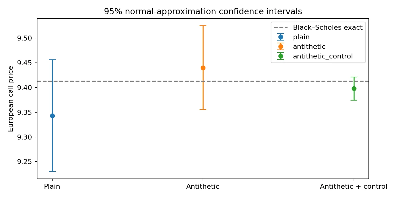
The blue markers are estimated call values; vertical bars show approximate sampling uncertainty. The dashed reference comes from the Black–Scholes formula for the same assumed inputs. These are simulated values—not live market quotes.
13. Interpreting the results instead of just celebrating a tiny error bar
The plotted estimators are:
- Plain Monte Carlo: independent discounted payoff samples.
- Antithetic Monte Carlo: independent pair averages, each built from and .
- Antithetic plus control: pair averages adjusted by the discounted-stock control.
You should see each price estimate near the analytic benchmark, within a plausible margin given its reported uncertainty. Sometimes a lower-variance method is farther from the correct price in a particular run: variance reduction improves behavior across repeated experiments, not guaranteed accuracy of every individual seed.
Also beware of comparing only the width of error bars. Record the number of underlying normal draws, option payoff evaluations, runtime, memory use and the assumptions used to estimate standard error. The sample-estimated control coefficient means its interval should be labeled approximate.
Can we see random error diminish as samples increase?
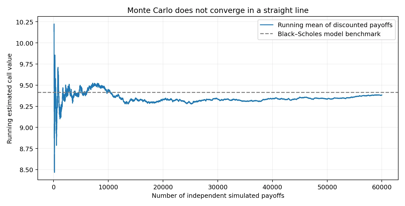
An illustrative reproducible run shows a plain Monte Carlo estimate as additional independent payoff samples accumulate. The wiggles are normal; convergence is statistical, not guaranteed to be monotone.
This chart is a useful antidote to a common misconception. Even when a method is consistent, the average may move away from the benchmark for a while before moving closer. The important pattern is that uncertainty tends to shrink with larger samples, not that every additional sample improves the answer.
14. Confidence intervals do not measure all pricing uncertainty
A narrow 95% Monte Carlo confidence interval answers a specific question: “How precisely did we calculate the option value under this assumed model and these inputs?” It does not answer “How accurate is the assumed model relative to market prices?”
Different sources of uncertainty need different responses:
| Problem | Example | Appropriate response |
|---|---|---|
| Sampling error | Too few independent scenarios | Increase samples or use variance reduction |
| Parameter uncertainty | Volatility estimate is wrong | Sensitivity analysis, calibration, alternative estimates |
| Model risk | Stock dynamics are not GBM | Alternative models, stress tests, market validation |
| Time-discretization error | Barrier crossing between simulated dates | Finer grids, bridge corrections, bias studies |
| Data/market frictions | Dividends, financing, bid–ask spread, liquidity | Realistic market inputs and execution assumptions |
Our European terminal call uses the exact GBM terminal distribution, so it does not introduce a time-stepping approximation for . A simulation of an Asian or barrier option generally depends on the path and can introduce time-discretization error; no number of simulated paths removes a systematic time-step bias.
15. Common beginner mistakes and how to catch them
Mistake 1: Averaging final stock prices instead of call
payoffs. The call is not the stock. Always apply
np.maximum(ST - K, 0) before averaging.
Mistake 2: Forgetting discounting. An expected payoff at is not automatically today’s price. Apply in this continuous-rate model.
Mistake 3: Using a personal stock-return forecast as the
risk-neutral drift. Physical expected returns and the
risk-neutral valuation measure are different concepts. Our
r comes from model-pricing assumptions, not a trading
prediction.
Mistake 4: Mixing annualized and daily inputs. If
is expressed in years,
and
must use consistent annualized units. A “20” volatility input means
2000%, not 20%; use 0.20.
Mistake 5: Computing a confidence interval using antithetic legs as independent observations. Use pair averages for the standard error.
Mistake 6: Trusting the narrowest result from one lucky seed. Use multiple independent seeds and compare estimated uncertainty with empirical variation across runs.
Mistake 7: Calling the estimated option value a real market quote. We use hypothetical input parameters. Real quoted option prices reflect instrument details, market liquidity, implied volatility structure, dividends/carry, and model limitations.
16. Four experiments to deepen your understanding
Experiment A — Change volatility. Price calls with and keep everything else fixed. Explain why the call price changes. Does the Monte Carlo confidence-interval width change too?
Experiment B — Move the strike. Try . Identify in-the-money, at-the-money and out-of-the-money calls. Which has more zero-payoff simulations?
Experiment C — Measure actual sampling variability. Run 30 independent seeds at and then at . Compare the distribution of sample means and nominal interval coverage. Does the typical error fall by approximately ?
Experiment D — Price an arithmetic Asian call. Replace the terminal payoff with a payoff based on the average stock price along a simulated path. Now the full path matters. Compare different time-step counts and discuss sampling error versus discretization bias. This extension is more realistic for learning path-dependent derivatives, but you must implement and validate it separately; our downloadable base program prices the simpler European call.
17. What you have actually learned
We began with the simplest possible question: what is a future right to buy a $100 stock for $100 worth today? A call’s payoff depends on the final price, so pricing it requires assumptions about a whole distribution of outcomes. In the Black–Scholes world, that distribution is risk-neutral GBM; Monte Carlo draws outcomes, discounts payoffs and averages them.
You can now explain what each mathematical symbol does, implement the pricing experiment, quantify Monte Carlo noise, check the answer against an exact reference and improve precision with antithetic and control variates. Just as importantly, you know where the conclusions stop: a precise simulated value under a hypothetical model is not proof of a real-world market price, trading edge or guaranteed investment return.
For a broader foundation, continue with Black–Scholes Model Explained or Monte Carlo Methods in Quantitative Finance. To identify what you understand and what to study next, explore the Algonique Quantitative Finance Skill Assessment.
Frequently asked questions
Can a beginner implement Monte Carlo option pricing in Python? Yes. If you understand averages, random numbers, and the call payoff, you can implement a first experiment. The advanced mathematics explains why the method is appropriate under particular assumptions and how to validate it.
Why use Monte Carlo when the Black–Scholes formula already exists? For this European call, the formula is a convenient correctness benchmark. Monte Carlo becomes especially useful for more complicated payoffs, multiple assets, and contracts where no convenient closed form is available.
Does a 95% confidence interval tell me the option’s market price? No. It approximates sampling uncertainty around the assumed model value. It does not include model misfit, volatility estimation, liquidity or future market movements.
Do antithetic variates always work? No. Whether they reduce variance depends on the payoff’s structure and the correlation between the paired outcomes.
What is a control variate in simple terms? It uses a second simulated quantity with a known true average to correct part of the accidental noise in the estimate you care about.
Do I need Itô calculus to run the script? No. The European-call experiment uses an exact formula for the GBM terminal stock value. Understanding Itô’s lemma helps explain the formula, but you can first learn the numerical workflow and return to the derivation later.
Can I use this script to decide whether an option is underpriced? Not directly. Our inputs are educational assumptions. Comparing with actual markets requires valid market data, calibrated parameters, correct contract specifications, and substantially more model and execution analysis.
Technical references
- NumPy: random number Generator — reproducible pseudorandom normal samples.
- NIST/SEMATECH Engineering Statistics Handbook — statistical estimation, uncertainty, and experimental reasoning.
- Black and Scholes (1973), The Pricing of Options and Corporate Liabilities — foundational mathematical pricing model.
- SciPy: normal distribution — reference implementation of the normal CDF if you want to extend the program.
Research disclosure: all figures in this article are simulations based on declared hypothetical parameters; they are not derived from historical option market quotes. The example does not contain actual trading, claims of arbitrage, or investment advice.