Semantic Search in Python: BM25 vs Embeddings vs Hybrid Retrieval — A Hands-On Benchmark
How would you build a search engine that understands a support
engineer asking “Why did we charge the customer twice?” but still finds
a precise incident code such as ERR-429? In this
beginner-friendly tutorial, you will implement and measure three
retrieval approaches instead of assuming the newest one wins.
Level: beginner to intermediate, with optional advanced sections. Tools: Python, NumPy, scikit-learn, optional Sentence Transformers. Estimated lab time: 30–60 minutes. What you will build: an inspectable local search benchmark with a BM25 ranker, a vector-embedding ranker, reciprocal rank fusion (RRF), 48 fictional technical documents, 22 labeled queries, metrics, timings, and visual diagnostics.
Research integrity: The included document collection and relevance judgments are authored educational examples, not production or public benchmark data. The default offline experiment uses TF-IDF followed by truncated SVD to produce low-dimensional LSA vectors, not pretrained neural embeddings. An optional second mode uses an actual Sentence Transformers model and requires installing the library and downloading model weights. All reported numbers below come from the reproducible offline LSA experiment, never from an unexecuted neural model. A tiny test cannot establish which system works best on your business data.
1. The real problem: one search box, two very different questions
Imagine an engineering team with hundreds of internal incident reports, payment playbooks, and operational runbooks. Everyone wants a single search box. Two employees type these queries:
- Query A:
ERR-429— the engineer knows the exact identifier of an inference-gateway error. - Query B: “Our customer paid, but the website timed out, and the second attempt charged them again.” — the support agent does not know the words “idempotency key” or “reconciliation.”
Both queries are reasonable. But they stress different capabilities.
Query A needs exact matching: an engine should not
replace ERR-429 with an article about generic slow
requests. Query B requires meaning matching: the best
document might be titled Duplicate charge after payment timeout
rather than containing the user’s exact sentence.
Here is a tiny fictional sample of the documents we will search:
| Document ID | Document title | Core idea |
|---|---|---|
SRV-001 |
ERR-429 on inference gateway | Respect rate limits and Retry-After. |
PAY-001 |
Duplicate charge after payment timeout | Check the original idempotency key before retrying. |
PAY-004 |
Idempotency key reuse | The same key must identify the same operation and payload. |
DB-002 |
Transactional outbox reliability | Record a database change and an outbox event atomically. |
ML-004 |
Embedding model mismatch | General embeddings can fail on specialized identifiers. |
The goal of search is retrieval: return a ranked list of relevant documents. This article does not pretend that retrieval alone is an answer-generating RAG assistant. An LLM might later summarize these documents, but if the right evidence was never retrieved, a fluent answer can still be wrong. For the complete downstream problem, read our RAG evaluation tutorial.
2. First, what does “relevant” mean?
Before choosing an algorithm, decide what counts as success. For
Query A, we explicitly label SRV-001 relevant. For Query B,
our small evaluation labels PAY-001 and
PAY-004 relevant. We write these labels
before assessing ranking quality. Otherwise we could
declare any result “good” after seeing what our favorite model
returned.
In a business search engine, these labels ideally come from multiple
reviewers who understand the actual task. A query can have several
relevant documents; some can be essential and others merely helpful. For
example, if the user asks how to prevent a duplicate charge,
PAY-001 explains the incident, while PAY-004
explains when reusing an idempotency key is safe. The first article
might answer the immediate question, but the second is necessary to
implement the fix safely. This is why we keep both labels rather than
choosing an arbitrary single “correct” document. You also need to record
cases where no answer exists, so the system learns to
abstain rather than fabricate a confident source.
A useful distinction is retrieval relevance versus
answer correctness. Returning PAY-001 may
be necessary for an agent to solve a payment issue, but the agent still
has to interpret the document correctly and follow authorized
procedures. That is a separate evaluation problem.
3. Start with keywords: why BM25 still matters
BM25 is a classic lexical search ranking function. Lexical
means that it matches words or tokens rather than directly comparing
semantic concepts. If a query contains ERR-429, a BM25
index can strongly reward a document containing precisely that
identifier.
Imagine scoring the query “payment timeout”. A document that mentions
payment and timeout repeatedly is a plausible
match. But repetition should not help forever: a 10,000-word page saying
“timeout” 200 times should not automatically beat a concise, directly
relevant incident report. And common words like “service” are less
informative than rare terms.
BM25 incorporates three intuitions:
- Term frequency: a matching query token can increase the score, but with diminishing returns.
- Document length: longer documents are adjusted so verbosity alone does not dominate relevance.
- Inverse document frequency: uncommon tokens tend to be more useful for distinguishing documents.
For a query and document , one common BM25 variant scores:
What do these symbols mean? is how often the token appears in the document; is the document length in tokens; is the average document length; controls the saturation of repeated terms; and controls length normalization. In our experiment we start with , . These are conventional starting values, not universal optima.
Our code uses the always-positive IDF convention:
where
is the number of documents and
is the number containing token
.
If ERR-429 is present in only one of 48 documents, its IDF
is much greater than a token appearing in almost all of them.
You do not need to memorize this equation to use BM25. The important practical insight is that lexical retrieval rewards exact, informative words and handles long documents carefully. For reference, see Elastic’s explanation of BM25.
An implementation you can read line by line
The downloadable project includes a tiny transparent BM25 implementation, so you can see rather than merely call the formula:
from collections import Counter
import math

def bm25_score(query_tokens, document_tokens, doc_frequencies,
               document_count, average_length, k1=1.5, b=0.75):
    counts = Counter(document_tokens)
    length = len(document_tokens)
    score = 0.0
    for term in set(query_tokens):
        freq = counts.get(term, 0)
        if freq == 0:
            continue
        docs_containing_term = doc_frequencies[term]
        idf = math.log(1 + (document_count - docs_containing_term + 0.5)
                       / (docs_containing_term + 0.5))
        normalizer = freq + k1 * (1 - b + b * length / average_length)
        score += idf * freq * (k1 + 1) / normalizer
    return score
This is the scoring calculation itself; the companion script adds tokenization, indexing and ranking for all 48 documents. The implementation is deliberately small enough to inspect and independently test. The five numerical inputs are not mysterious hyperparameters: they come directly from counts collected while indexing the document collection.
Important tokenizer detail: our tokenizer preserves
IDs containing hyphens, such as ERR-429, as a single token.
In a real search application, tokenization, casing, punctuation,
synonyms and language-specific stemming deserve their own tests. If a
tokenizer breaks an important product identifier, the best ranking
formula cannot repair the lost information.
4. Why keywords alone can fail
Suppose an engineer searches: “How can our backend avoid sending an event when a database transaction fails?” The relevant document is about a transactional outbox. It may use terms such as atomic persistence, publish, and outbox, while the searcher says send and fails. A purely lexical retriever may miss the conceptual match, especially if there are few overlapping words.
The same happens with abbreviations, regional spelling, paraphrases, and vocabulary gaps between newcomers and subject-matter experts. However, do not overstate this weakness: keyword systems can be enhanced with synonym dictionaries, field boosting, query rewriting and domain-specific analyzers. BM25 is a strong baseline, not a primitive straw man.
The question is whether we can represent the meaning or latent structure of a text more flexibly than exact-token overlap.
5. What is a text embedding? Start with a three-number example
A vector is simply an ordered list of numbers. Imagine a deliberately simplified embedding space with three dimensions:
| Text | Payments | Reliability | Databases |
|---|---|---|---|
| “Prevent a second charge after timeout” | 0.9 | 0.7 | 0.1 |
| “Idempotent payment requests” | 0.9 | 0.8 | 0.1 |
| “Database vacuum and table bloat” | 0.0 | 0.1 | 0.9 |
These three numbers are invented to explain the idea; they are not the output of our model. The first two texts point in a similar direction even though they use different words. The last one points elsewhere.
Modern embedding models produce hundreds or thousands of learned numerical features. Their individual dimensions are usually not labeled “payments” or “reliability.” We compare vectors by a geometric similarity measure, commonly the cosine:
Consider two tiny unit-length vectors: and . Their dot product is , so their cosine similarity is 0.8. For a perpendicular vector , it is 0.0. This elementary geometry is all you need to understand the final similarity comparison; the hard part is learning a representation in which useful meanings are close together.
The numerator is the dot product; the denominator normalizes for vector length. When both vectors have unit length, cosine similarity is simply their dot product. A larger score signals that the encoded query and document point in more similar directions.
Two different ways to construct embeddings
A. Classical latent semantic analysis (LSA). We calculate TF-IDF features for our training corpus, then use truncated singular value decomposition (SVD) to project them into a smaller numerical space. This creates low-dimensional vectors and exposes some latent word co-occurrence structure. It runs offline, quickly, and is excellent for teaching linear algebra and vector retrieval. But it is not a pretrained neural semantic model. It often struggles when a synonym was never used in a shared textual context.
B. Pretrained sentence embeddings. A model such as
sentence-transformers/all-MiniLM-L6-v2 encodes text with
parameters learned from broader training data. It can sometimes connect
paraphrases that rarely co-occur in our tiny dataset. It can also fail
on precise IDs, specialized financial jargon, negation, or ambiguous
wording. Performance must be measured rather than assumed.
The Sentence
Transformers documentation distinguishes symmetric and asymmetric
retrieval. For short questions searching longer documents, it recommends
encode_query() and encode_document() where
supported by the selected model.
Our project implements both modes and labels all outputs with the encoder used. The printed LSA metrics must not be described as a neural-embedding benchmark.
6. Build the local experiment step by step
The bundled collection has 48 fictional technical documents across payments, operations, databases, machine learning, finance and security. There are 22 manually authored queries: six exact identifiers, twelve natural-language paraphrases, and four mixed queries. Some queries have more than one relevant answer. All data is included as Python source; there is no paid API, hidden dataset, external search engine or database requirement for the offline experiment.
Each document has an ID, title, body and topic; each query has an ID, text, relevance labels and query group. The project freezes these inputs so everyone can reproduce the same educational measurement.
# Simplified illustration of the bundled data format:
Document(
    id="PAY-001",
    title="Duplicate charge after payment timeout",
    text="If the provider accepted the charge but the HTTP response was lost...",
    topic="payments",
)

("q07", "My customer was charged twice after the request timed out...",
 {"PAY-001", "PAY-004"}, "paraphrase")
What this dataset does not prove: forty-eight short documents do not represent the scale, document length, language variety, ambiguity or access-control constraints of a company knowledge base. Our labels are illustrative, not independently adjudicated. We are teaching how to evaluate a retrieval pipeline, not publishing a leaderboard.
7. Implement the vector branch in Python
First, the offline LSA branch. It combines two standard scikit-learn steps:
vectorizer = TfidfVectorizer(
    ngram_range=(1, 2),
    sublinear_tf=True,
    stop_words="english",
)
X = vectorizer.fit_transform(document_texts)

svd = TruncatedSVD(n_components=32, random_state=42)
doc_vectors = normalize(svd.fit_transform(X))

query_vector = normalize(svd.transform(vectorizer.transform([query])))[0]
scores = doc_vectors @ query_vector
The TF-IDF vectorizer is fitted on documents, not on
future test questions. The query uses transform, not
fit_transform: it is projected into the already defined
feature space. The SVD likewise learns its basis on documents only. That
is what a real retrieval system does: it indexes documents independently
from the query it is about to receive.
This is also why new query words absent from the document vocabulary may vanish in LSA. You are seeing an important limitation of corpus-trained representations, not a bug.
Switch to actual pretrained sentence embeddings
Once you have installed the optional dependencies and downloaded a model, use the same document collection, labels and evaluation function:
from sentence_transformers import SentenceTransformer

model = SentenceTransformer("sentence-transformers/all-MiniLM-L6-v2")

doc_vectors = model.encode_document(
    document_texts,
    normalize_embeddings=True,
    convert_to_numpy=True,
)
query_vector = model.encode_query(
    [query],
    normalize_embeddings=True,
    convert_to_numpy=True,
)[0]
scores = doc_vectors @ query_vector
The model must download weights on first use unless you have cached them. The neural mode is therefore optional and not validated by the offline numbers in this article. Results vary with the selected model, library version and hardware. For production use, verify embedding dimensionality, text truncation behavior, prompt conventions and any external data transfer.
8. Why raw BM25 scores and cosine scores should not be added
BM25 scores are unbounded positive relevance scores (their magnitude
depends on corpus statistics and tokenization). Cosine similarities for
unit vectors are in approximately
.
A plain 0.5 * bm25 + 0.5 * cosine can make the lexical
score dominate just because its numeric scale is different. The choice
of normalization is itself a modeling decision.
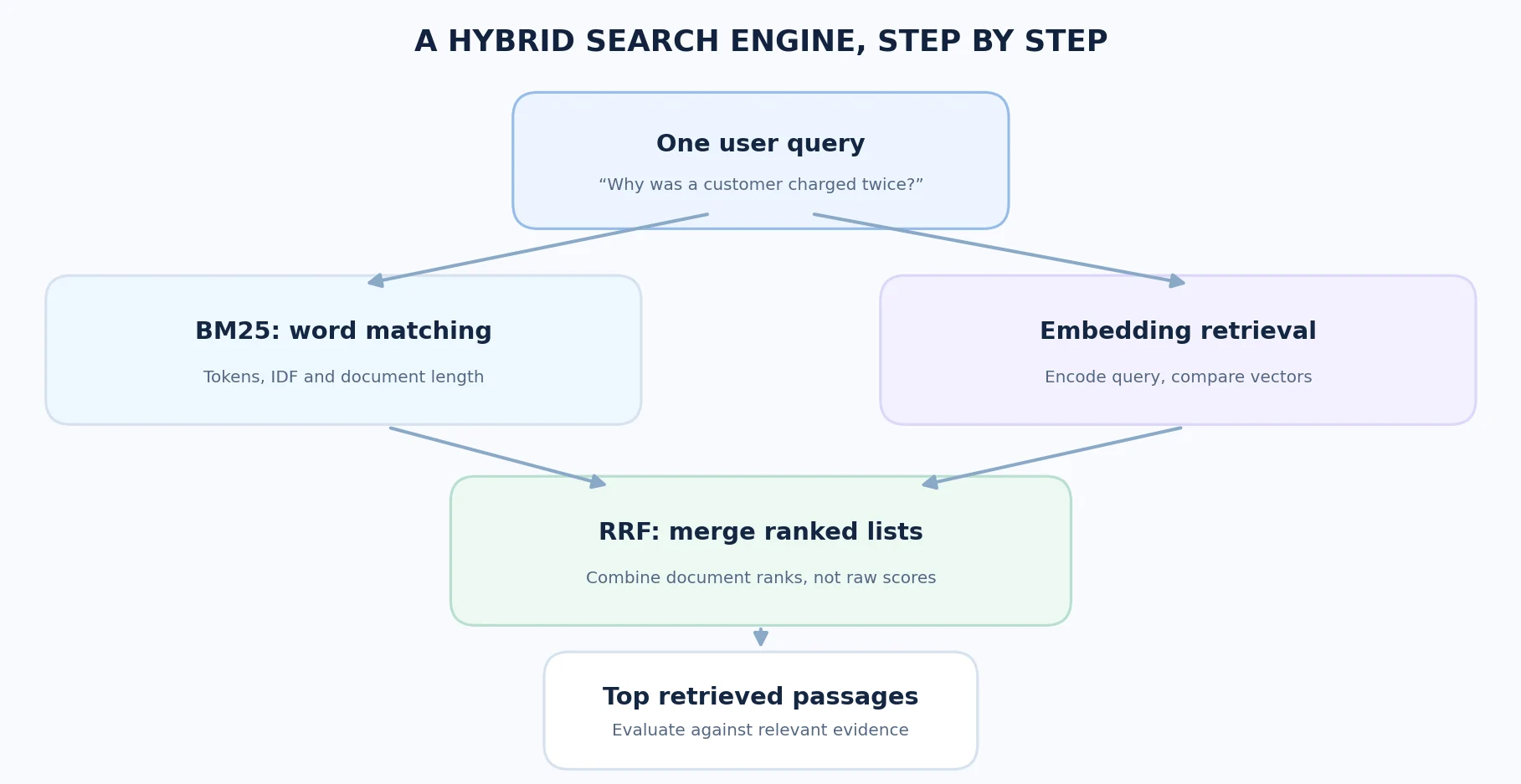
A simple alternative is reciprocal rank fusion, or RRF. Instead of adding raw scores, combine the positions of a document in two ranked lists:
A commonly used starting constant is . If a document ranks first under BM25 and third under vectors, its combined score is:
Imagine another document ranks second in BM25 but never appears in the vector top-20 candidates. Its score is only . Our first document’s is almost twice as large because both methods found it near the top. That does not prove the first document is relevant, but it explains the mechanism without requiring you to understand any vector coordinates.
For an operational counterexample, suppose a very rare exact error code produces a perfect BM25 result, while the vector model returns many generic “server errors” articles. RRF might then push an irrelevant generic article above the exact-code article, especially if several branches or candidate limits are changed. Hybrid must be tested on exact-code queries before deployment, not added as a default assumption.
It is the agreement of two rankings, not their incompatible raw scoring units, that pushes a document upward. This idea was introduced in a 2009 information-retrieval paper by Cormack, Clarke and Büttcher.
Our implementation is short enough to inspect:
def rrf(rankings, k=60, top_n=10):
    combined = {}
    for ranked in rankings:
        for position, doc_id in enumerate(ranked, start=1):
            combined[doc_id] = combined.get(doc_id, 0) + 1 / (k + position)
    return sorted(combined, key=lambda d: (-combined[d], d))[:top_n]
Each retrieval branch contributes only its top 20 candidates in the experiment. The BM25 branch omits documents with a zero lexical score; otherwise arbitrary zero-score ties would artificially enter the fusion pool. RRF does not guarantee that the final ranking improves. Two systems can agree on irrelevant documents, or one good system can be diluted by a weaker partner.
9. Evaluate retrieval with metrics rather than attractive examples
You need a dataset of labeled queries; otherwise a screenshot of one successful answer proves very little. Three metrics are especially helpful.
Recall@K: did we find enough of the relevant documents?
If two documents are relevant and only one is returned in the top three, Recall@3 is . This matters in RAG: the generator might need two pieces of evidence, not merely one.
MRR@K: how quickly did the first good result appear?
where is the rank of the first relevant document. If it appears first, the reciprocal rank is 1; if third, it is . Mean reciprocal rank (MRR) averages these values over the questions. MRR is useful for tasks where one strong result is enough, but it ignores whether additional relevant documents were returned.
Latency: how long did retrieval take?
Query latency determines how responsive a system feels. Measure the steady-state search path separately from expensive one-time indexing or neural-model loading. Also measure the end-to-end system in production: network, metadata filters, ANN retrieval, reranking, and content fetch can be much more important than a few hundred microseconds in an in-memory toy program.
We report median single-process query times over 50 repeated runs, on only 48 documents. They are educational timing measurements, not production service-level estimates. The evaluation exports a CSV with each query, top-ranked documents, relevance labels and per-query metrics so you can audit the result.
10. The actual offline benchmark: sometimes hybrid is better, sometimes not
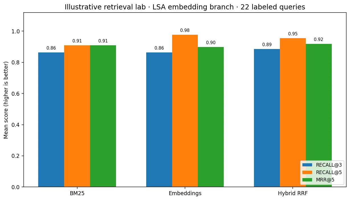
We ran
python semantic_search_lab.py --encoder lsa --output output
on the included 48-document, 22-query fictional dataset. Here are the
measured offline LSA-mode results, rounded to three
decimals:
| Retrieval system | Recall@3 ↑ | Recall@5 ↑ | MRR@5 ↑ |
|---|---|---|---|
| BM25 | 0.864 | 0.909 | 0.909 |
| LSA vector retrieval | 0.864 | 0.977 | 0.899 |
| BM25 + LSA hybrid RRF | 0.886 | 0.955 | 0.918 |
The actual script writes full precision and per-query
measurements to output/metrics.json and
output/query_results.csv. These are not real company
searches or results from a downloaded transformer.
What do the results actually mean?
- LSA wins Recall@5 in this particular sample. It retrieved slightly more of the known relevant documents within five results.
- Hybrid has a slightly stronger MRR@5. Across these authored questions, the first relevant document was placed a little earlier on average.
- BM25 remains strong. In our exact-identifier question group, its MRR@5 was 1.0. It is risky to replace it solely because “vectors sound modern.”
The differences are small, the dataset is tiny, and the examples were written by the experiment author. None of these numbers establishes that hybrid retrieval is superior in an independent production setting. That is exactly the right lesson: select methods based on labeled evaluation data and realistic failure costs.
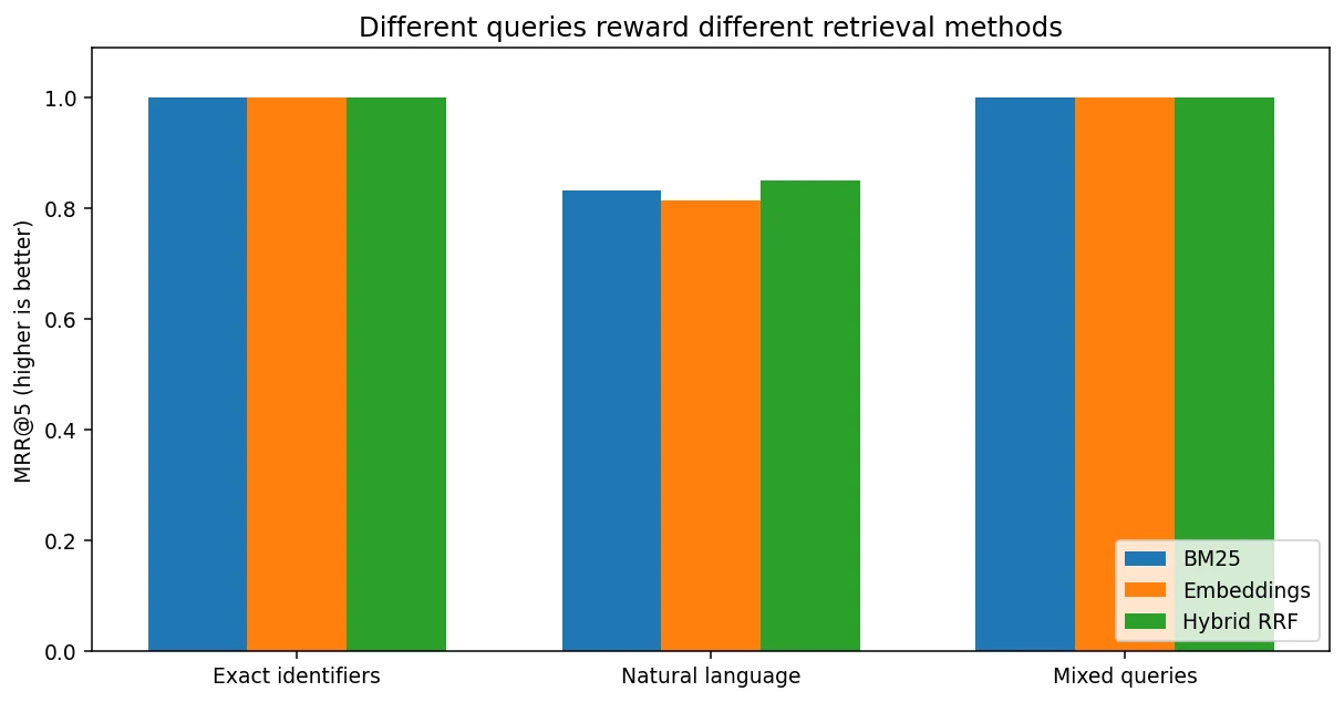
A search team should also measure cases where the only relevant result is ranked beyond the cutoff, user satisfaction on live queries, how well the system respects permissions, and whether retrieved passages actually support downstream answers. For larger evaluations, see the BEIR evaluation framework and available metrics.
11. Walk through an actual ranked result
Let’s inspect our Query 7: “My customer was charged twice after the
request timed out…” The manually labeled relevant documents are
PAY-001 and PAY-004.
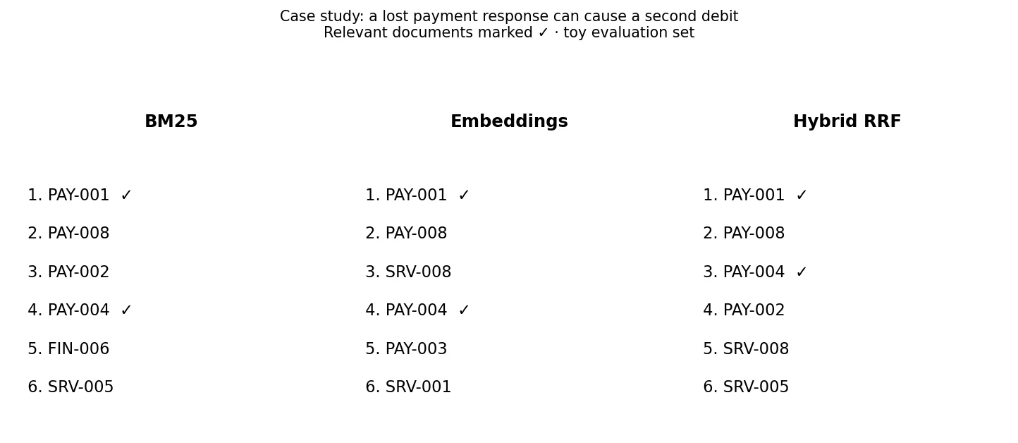
Instead of just comparing a final accuracy number, this diagram shows
the top six retrieved document IDs per approach,
marking relevant ones. This lets us ask why something was
ranked: Did BM25 reward the exact words charged and
timeout? Did the vector branch move an idempotency document
earlier? Did RRF demote a relevant candidate from one branch?
This inspection is as important as aggregate metrics, especially if a search system is feeding an AI agent that could make financial or security-sensitive decisions. Human-readable IDs and query-level CSV traces make debugging possible.
12. Latency: what we measured and what we did not
The project also measures steady-state per-query ranking time using the same machine and single query, in a loop. On the author’s isolated environment, one run produced approximately:
| Method | Median query time, milliseconds |
|---|---|
| BM25 | 0.217 |
| LSA vectors | 0.377 |
| Hybrid RRF | 0.666 |
These times are so small because the corpus fits in RAM and no network is involved. They exclude model loading, document ingestion, index construction, API calls and concurrency. A transformer implementation will have very different inference costs from LSA, so the table should never be used to compare neural search performance without running the neural mode.
A real deployment should measure p50/p95/p99 end-to-end latency, index-refresh overhead, memory usage, and search throughput at realistic corpus sizes. When the corpus grows, an approximate-nearest-neighbor (ANN) index may be appropriate, but that introduces a separate recall-versus-speed tradeoff.
13. Run the entire project yourself
The downloadable package contains corpus.py,
semantic_search_lab.py, requirements.txt, an
optional transformer requirements file, and automated tests. It does not
require credentials or external APIs for offline LSA mode.
python3 -m venv .venv
source .venv/bin/activate       # Windows: .venv\Scripts\activate
python -m pip install -r requirements.txt

# Completely offline illustrative comparison:
python semantic_search_lab.py --encoder lsa --output output

# Automated checks:
python -m pytest -q
The script generates output/metrics.json,
output/query_results.csv and three reproducible figures. To
compare real pretrained sentence embeddings, run:
pip install -r requirements-transformer.txt
python semantic_search_lab.py \
  --encoder transformer \
  --model sentence-transformers/all-MiniLM-L6-v2 \
  --output output-transformer
The transformer step requires an internet connection on first use and can take longer. It is a separate experiment. Keep the output directories distinct; never overwrite offline-LSA charts with neural charts without updating their captions and metadata.
14. Five mistakes that make search benchmarks misleading
Mistake 1: Inventing relevance after seeing the results. Define and review search relevance first. When evaluating a new method, use a held-out query set that was not repeatedly inspected and optimized against.
Mistake 2: Calling TF-IDF or LSA “a state-of-the-art semantic embedding model.” Both are useful vector representations; neither is interchangeable with a pretrained sentence-transformer. Label architectures and datasets accurately.
Mistake 3: Mixing scores without scale awareness. Raw BM25 and cosine scores are not numerically comparable. Use a justified score normalization, rank fusion, or a trained reranker with proper evaluation.
Mistake 4: Ignoring exact identifiers and security filters. Similar vectors are not a substitute for exact SKU matching, policy version constraints, tenant boundaries, ACLs, or time-validity filters. Retrieval can be semantically plausible but operationally unacceptable.
Mistake 5: Using toy latency as a production performance claim. An in-memory evaluation says little about a distributed vector store, network latency, approximate retrieval, document storage or p99 under load.
There is an additional subtle error: retrieval evaluation leakage. If you repeatedly edit your dataset and relevance labels based on the rankings you see, you are gradually optimizing to the benchmark rather than measuring generalization. Create separate development and final test query sets when the research becomes serious.
15. From this experiment to production retrieval
A real knowledge system requires far more than two score functions. Start with your actual data: ingestion, document parsing, chunking, versioning, deduplication, metadata and permission checks. Build a query log from real tasks after appropriate privacy safeguards. Annotate relevance with clear criteria and multiple reviewers for difficult queries.
Then compare stronger baselines: a production lexical engine (BM25 with analyzers and field weighting), a neural bi-encoder appropriate to your language and domain, hybrid RRF, and optionally a cross-encoder reranker. Tune candidate counts and RRF parameters on development queries; reserve independent test queries for final comparisons.
Consider a candidate + reranker architecture: retrieve perhaps 50–100 documents cheaply, then apply a more expensive pairwise or cross-encoder model to reorder those candidates. This often improves relevance, but it also adds latency and operational complexity; the empirical tradeoff is task-specific.
For sensitive assistants, test whether the system honors authorization boundaries before results reach the language model. Retrieving one forbidden document and hoping the generator ignores it is not an adequate security design.
For RAG applications, measure the entire chain: retrieved-evidence recall, citation correctness, answer factuality, abstention quality and resistance to instruction text embedded in retrieved documents. The Reliable AI Agent tutorial explains why tool outputs and external content must be treated as untrusted data.
16. Practice exercises that build real retrieval intuition
Exercise A — Exact-code failure. Add two documents
that differ only by ERR-429 versus ERR-493 and
verify that your tokenizer and scoring preserve the distinction. Check
whether the transformer mode behaves differently.
Exercise B — Synonym mismatch. Create a document about loan installments and query for debt payments. Compare BM25, LSA and a pretrained sentence transformer. Do not assume which will win.
Exercise C — Hybrid tuning. Try RRF candidate limits of 5, 20 and 40 and constants of 10, 30 and 60. Explain why the differences must be evaluated on held-out queries, not merely selected for the nicest demo.
Exercise D — Negative queries. Add questions for which your corpus contains no evidence. Design an explicit “insufficient evidence” response rather than forcing a best match.
Exercise E — Latency at scale. Grow the corpus to thousands of documents and separate index-building costs from query costs. If you add ANN, measure approximate recall relative to brute-force cosine search.
17. Conclusion: use the right retrieval tool for the right problem
BM25 is a valuable tool when exact words and identifiers matter. Embeddings offer a different retrieval signal that can help with paraphrases and conceptual matching, depending on the model and data. Hybrid retrieval combines signals, but combining signals does not guarantee better results.
The key engineering skill is not remembering which algorithm is fashionable. It is being able to define relevance, build repeatable experiments, interpret metrics, investigate individual failures, and account for latency, security and data quality. That is what turns a retrieval demo into a reliable search system.
If you enjoyed debugging and measuring retrieval rather than simply calling an AI API, explore our RAG evaluation guide, LLM evaluation tutorial, and AI Skill Assessment to test your understanding of information retrieval, machine learning and production AI systems.
Frequently asked questions
Is BM25 obsolete now that we have embeddings?
No. Exact terms, structured identifiers, legal citations, software error codes and technical jargon can favor lexical retrieval. Both methods should be evaluated against the same tasks, with relevant documents labeled before comparing them.
Does hybrid search always beat pure BM25 or dense retrieval?
No. Our own small educational benchmark has the highest Recall@5 for LSA vectors, while hybrid ranks first on MRR@5. Different metrics and datasets reward different behavior.
Are TF-IDF and LSA the same as modern sentence embeddings?
No. TF-IDF is a lexical feature representation; LSA compresses it into a low-dimensional latent space. A pretrained sentence-transformer learns vector representations from a wider training process. All produce numbers, but their learning mechanisms and retrieval strengths differ.
What is the difference between Recall@5 and MRR@5?
Recall@5 asks how many relevant documents are in the first five results. MRR@5 asks how early the first relevant document appears, averaged across queries. A system can improve one metric and worsen the other.
Why use RRF instead of averaging BM25 and cosine similarity?
Their raw scores have different scales. RRF combines ranking positions, avoiding the need to add numerically incompatible values directly. It still requires careful candidate selection and evaluation.
Can I use this directly with my company’s private documents?
As an educational starting point, yes, after replacing the fictional corpus and labels. Production requires document access control, query privacy, secure data handling, long-document chunking, monitoring and relevance evaluation on actual tasks. Do not treat the toy script as a hosted secure search service.